| |
Multiple Linear Least Squares (MLLS) Fitting in EELS analysis matchs the measured spectrum
to several components. However, in this case,
the amount of additional data needed is much more than
a single number. The MLS procedure has become available in commercial software and deserves to
be used more frequently than in the past [5]. Multiple linear least squares (MLLS) fit technique has many applications:
i) To evaluate the atomic percentages of each element by computing the relative fit weights and integrating the references over an energy range.
ii) To interpret the elemental maps and/or EEL spectra due to overlapping edges (e.g. Table 1389). In EELS quantification, if the edges from different elements are too close and thus the peaks overlap, then the conventional edge intensity extraction is not possible. In this case, the MLLS deconvolution can be used to fit suitable standard (reference) spectra to all overlapping edges, and thus the overlapping edges can be effectively separated. However, if the edge onsets are extremely close (e.g., for the case of Ga/Si in Table 1389), the measurement accuracy will be affected by the change of bonding environment.
| Table 1389. Deconvolution examples of EELS overlap peaks by using MLLS fit technique. The energy range is used to perform MLLS fit. |
Edge separation between edges (eV) |
Overlap peaks |
Energy range (eV) |
Reference
|
| Element A |
Element B |
Symbol |
Edge (eV) |
Window used for signal (eV) |
Symbol |
Edge (eV) |
Window used for signal (eV) |
| 42 |
Pb |
N7,6: 138 |
145-240 |
Zr |
M5,4: 180 |
180-240 |
145-240 |
[2] |
| 43 |
Cr |
L3,2: 575 |
|
O |
K: 532 |
|
|
[3] |
| 4 |
Si |
L3,2: 99 |
|
Ga |
M3,2: 103 |
|
|
|
iii) To analyze the fine structure of EELS SI (spectrum image) in order to map out the relative intensities associated with a number of chemical states of core loss edges, e.g. Cu (Cu0+ and Cu2+) and Mn (Mn3+ and Mn4+). The advantage of the MLLS fit technique is that it is able to differentiate the small separation between the primary peaks from different valence states.
iv) To improve the EELS detection limit and weak signal extraction. For instance, by using the MLLS fit technique instead of conventional background subtraction, Cr concentrations as low as 0.03% in Al2O3 was possibly detected at a particular microscope setting. [1]
For the single scattering spectrum, the overall intensity of the spectrum can be given by a power-law background and core-loss profile for each edge:
I(E) = AE-r + C1IC1(E) + C2IC2(E) + ... + CNICN(E) -------- [1389]
where,
AE-r -- Power-law background fit.
C1 - CN -- Weightings of the
contribution of each element.
I1(E) - I N(E) -- Intensity of the
contribution of each element at an energy E.
The core-loss profiles can be calculated using elemental standards of known thickness
and composition. Or, a more accurate way is that the profiles are measured experimentally. In multiple least-squares (MLS)
fitting, the weightings of the
contribution of each element are adjusted by and their values converted to relative concentrations.
Such standard spectra used in the MLLS fit technique are acquired from reference specimens. The selection of proper references is crucial to the success of the MLLS fit method. Furthermore, for accurately quantitative analysis, spectra obtained from different valence states should be used as references. Therefore, MLLS depends
on fitting a sum of reference spectra, usually a Power law
background (or any background model) and one or more isolated
ionization edges, to a measured spectrum.
As an example, the procedure of using MLLS fit to deconvolute O K edge and Cr L2,3 edges is:
i) Standard
(reference) spectra with background, oxygen, chromium signals, obtained from alumina and chromium films, are measured under identical conditions to the source spectra and are normal
ized to the integrated counts within 100 eV above the edge onset. In this case, the fitting coefficients obtained with the MLLS fit
are equal to the estimated signals in the
source spectra.
ii) The background in front of the O K edge was modeled using power-law fit, starting immediately in front of the edge.
iii) The MLLS fit is performed including the background function and reference edges.
Figure 1389 shows the oxygen (O) elemental maps obtained with both power-law fit and multiple linear least-squares fit. The measured materials is Ca/TiO.
It shows that the extracted net intensities in the area on right-hand side differ by as much as 30%, and the O map obtained with MLLS fit can differentiate the oxygen levels in different areas clearer than that with power-fit.
.
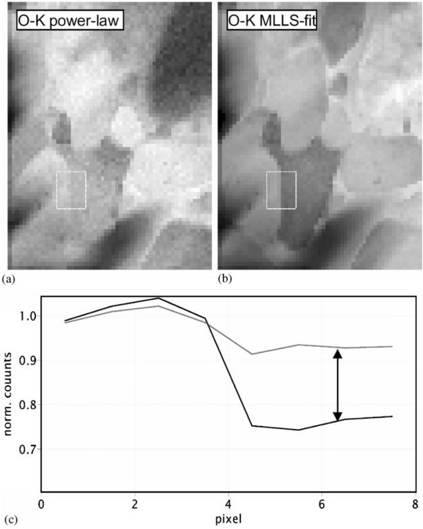
| Figure 1389. Oxygen elemental maps obtained with power-law fit (a) and multiple linear least-squares fit (b).
The extracted net intensities differ by as much as 30% (c). The measured materials is Ca/TiO. [4] |
However, it is necessary to note that inaccuracy from MLLS fit can be introduced because uncertainties, e.g. shape difference between the reference spectrum and the analyzing spectrum, exist over the fitting region which is not necessarily the same region used to extract the signal.
[1] Riegler, K.; Kothleitner, G.: EELS detection limits revisited: Ruby — a case study, Ultramicroscopy 110 (2010) , S. 1004 – 1013.
[2] Harkins, P. and MacKenzie, M. and Craven, A.J. and McComb, D.W. (2008) Quantitative electron energy-loss spectroscopy (EELS) analyses of lead zirconate titanate. Micron, 39 (6). pp. 709-716. ISSN 0968-4328.
[3] Katharina Riegler, and Gerald Kothleitner, EELS detection limits revisited: Ruby — a case study, Ultramicroscopy 110, 1004–1013, (2010).
[4]
Gerald Kothleitner and Ferdinand Hofer, Elemental occurrence maps: a starting point for quantitative EELS spectrum image processing, Ultramicroscopy 96, 491–508 (2003).
[5] R.F. Egerton, New techniques in electron energy-loss spectroscopy and energy-filtered imaging, Micron 34 (2003) 127–139.
|
|