A. Lenz Model for Elastic Scattering Distribution
In the literature, various relatively simple models of elastic electron–electron scattering such as a free-atom Thomas–Fermi
model with partial wave expansion [7]
and Mott cross-sections for a screened Coulomb potential
[8] had been proposed. On the other hand, Lenz model is a very simple atomic model. In this model, the single elastic scattering distribution is
given by [1, 3],
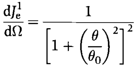 ------------------------- [964a] ------------------------- [964a]
where,
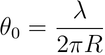
here, θ0 -- the characteristic screening angle of elastic
scattering. For the
binary materials, θ0 is taken as the mean characteristic
angle of each element weighted by the atomic fraction.
R -- is the screening radius of
atomic electrons ( 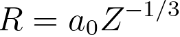 ). ).
Z -- the atomic number for a single element, or the effective atomic number for a component.
λ -- the electron wavelength,
a0 -- the Bohr radius.
Noted that θ0 ≈ 100θE. Here, θE stands for the characteristic angular range of inelastically scattered electrons as given by θE = E/γm0v2 with the usual relativistic factor γ.
Based on Figure 964, the relationship between the scattering angle and vector of the electron wave can also be given by the scattering vector q,
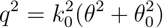 ------------------------- [964b] ------------------------- [964b]
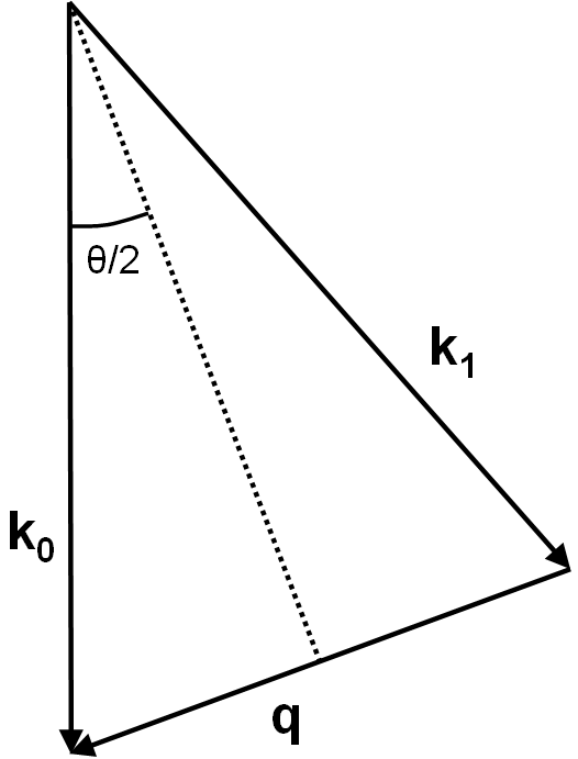
| Figure 964. Initial (k0) and final
(k1) wave vector of an elastically scattered electron and momentum transfer q. |
The elastic differential cross-section in the Lenz model can be given by,
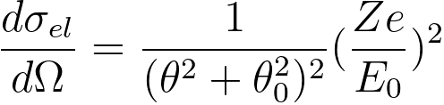 ------------------------- [964c] ------------------------- [964c]
where,
e -- the elementary
charge,
E0 -- the energy of the incident electrons.
In combination of Equations 964a and 964c, one is able to obtain,
 ------------------------- [964d] ------------------------- [964d]
The Lenz model can also give the elastic-scattering intensity dIe
within an angular range dθ by, [5]
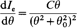 ------------------------- [964e] ------------------------- [964e]
where,
C - a constant.
B. Lenz Model for Inelastic Scattering Distribution
Lenz model gives the differential cross-section for electron–electron inelastic scattering as, [9]
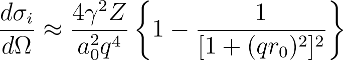 ------------------------- [964f] ------------------------- [964f]
where,
 , the scattering vector of inelastic scattering, , the scattering vector of inelastic scattering,
 , a
scattering angle, corresponding to a mean energy loss, which is usually denoted
as the characteristic angle for inelastic scattering. Because the majority of the energy
losses is normally below 100 eV, the characteristic angle is of the order of a few tenths
of a mrad, which is much smaller than typical Bragg angles in electron diffraction patterns of crystals. For instance, for 200 keV electrons, , a
scattering angle, corresponding to a mean energy loss, which is usually denoted
as the characteristic angle for inelastic scattering. Because the majority of the energy
losses is normally below 100 eV, the characteristic angle is of the order of a few tenths
of a mrad, which is much smaller than typical Bragg angles in electron diffraction patterns of crystals. For instance, for 200 keV electrons,  (mrad), here the mean energy loss, (mrad), here the mean energy loss,  , is in eV. , is in eV.
In practice, the simple Lenz atomic model of scattering suggested that the cross section (per atom) for inelastic scattering can be given by a power-law dependence,
 --------------------- [964g] --------------------- [964g]
However, more sophisticated calculations suggested: [4]
 --------------------- [964h] --------------------- [964h]
The exponent x actually depends on collection semi-angle.
As it can be seen above, this relatively simple Lenz model provides an estimate of the atomic DCS (differential cross section).
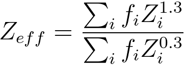
C. Effective atomic number in Lenz model
In the Lenz model, the atomic number of a compound can be approximated
using an effective atomic number Zeff, [9]
 --------------------------------------- [964i] --------------------------------------- [964i]
where,
fi -- the atomic fraction of each element of atomic number Zi.
Equation 964i can be computed with a DM script. Note that for approximate EELS calculations, an estimate of the 'mean' Z of the region under
investigation can often suffice.
D. Summary
The Lenz
atomic model shows that:
i) the Lenz
values are mostly higher than the experimental ones at low angles,
but lower at high angles (no objective aperture). [6]
ii) the consideration of multiple scattering and aperture effects (represented by θ) is important to the correct interpretation of an energy-loss
spectrum.
iii) the cross-sections increase with atomic number roughly as Z1/3 as shown in Equation 964g.
The Lenz
atomic model predicted that:
i) the total cross section per atom σt increases with increasing atomic number. [6]
The elastic Lenz model had been used to:
i) correct the effects of elastic scattering in amorphous materials. [1] However, since the Lenz model is atomic in nature and thus it does not
account for solid-state effects such as Bragg scattering and channelling.
ii) calculate the effective contrast thickness in transmission electron microscopy. [2]
iii) discuss the effects of elastic
scattering on the core-loss and low-loss electrons. [1]
Note that as shown in Table 964, other models have to be employed in order to account for the influence of plural scattering on the EELS elemental analysis of thick specimens due to the effect of multiple electron scattering.
Table 964. Single and multiple electron scattering.
[1] K. Wong and R. F. Egerton, Correction for the effects of elastic scattering in core-loss quantification, Journal of Microscopy, 178(3), (1995) pp. 198-207.
[2] L. Reimer, Transmission Electron Microscopy, Physics of Image Formation, and Microanalysis (Springer, Berlin, 1989).
[3] F. Lenz, Z. Naturforsch. Teil A 9, 185 (1954).
[4] Crewe, A.V., Langmore, J.P., and Isaacson, M.S. (1975) Resolution and contrast in the scanning electron microscope. In: Physical Aspects of Electron Microscopy and Microbeam Analysis. B.M. Siege1 and D.R. Beaman, eds. Wiley, New York, pp. 47-62.
[5] S. C. Cheng and R. F. Egerton, Elemental Analysis of Thick Amorphous EELS, Micron, Vol. 24, No. 3, pp. 251 256, (1993).
[6] Huai-Ruo Zhang, Ray F. Egerton, Marek Malac, Local thickness measurement through scattering contrast and electron energy-loss spectroscopy, Micron 43 (2012) 8-15.
[7] Ichimura, S., Aratama, M., Shimizu, R., Monte Carlo calculation
approach to quantitative Auger electron spectroscopy. J. Appl. Phys.
51, (1980) 2853–2860.
[8] Shimizu, R., Kataoka, Y., Matsukawa, T., Energy distribution
measurement of transmitted electrons and Monte Carlo simulation for
kilovolt electron. J. Phys. D 8, (1975) 820–828.
[9] R.F. Egerton, Electron Energy Loss Spectroscopy in the Electron Microscope (NewYork, Plenum Press, 1986).
|