=================================================================================

Newton's method is an optimization algorithm used in machine learning and various other fields to find the minimum or maximum of a real-valued function. It is an iterative method that converges quickly to the optimal solution when the function is well-behaved, particularly when it is smooth and convex.

Newton's method is often employed for solving optimization problems, such as finding the parameters (weights) of a model that minimize a loss function. Here's a high-level overview of how Newton's method works:

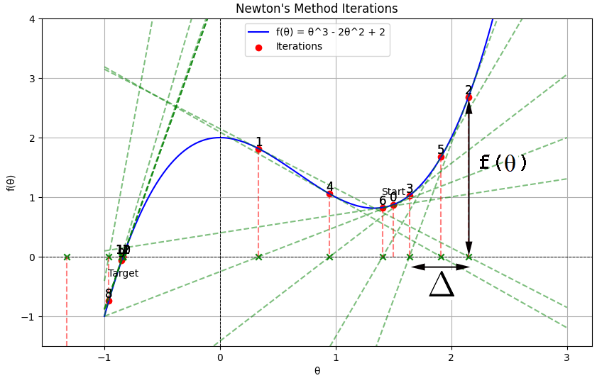
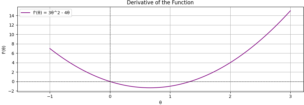
Figure 3873 illustrates Newton's method by its key principles and the derivative of the function of the curve. The derivative of function f(θ) can be given by,

--------------------------------- [3873a]

where,

          Δ is the distance along x-axis, e.g. from the projected dot, on x-axis, of the point 2 to the intersect at x-axis, which is used to form point 3 on the curve as the next step of Newton's method.

          f(θ) is the height from the curve.

Then,

--------------------------------- [3873b]

And, we have:

          --------------------------------- [3873c]

Therefore, we have:

--------------------------------- [3873d]

...

--------------------------------- [3873e]

Assuming,

          --------------------------------- [3873f]

Then, we have:

          --------------------------------- [3873g]

In the above discussion, θ is real numbers. However, when θ is vectors, then we have:

--------------------------------- [3873h]

Where:

• x_k​ is the current estimate of the solution.
• α is a step size or learning rate.
• ∇f(x_k) is a vector which is the gradient of the objective function at x_k.
• H_f(x_k) is the Hessian matrix (second-order derivative) of the objective function at x_k:

                              ------------------------------- [3873i]

Newton's method can be used to find a solution (θ) to the equation f(θ) = 0 and its derivative ℒ'(θ) = 0. In this case, ℒ(θ) represents a loss or cost function typically used in machine learning or optimization problems.

The detials of Figure 3873 are:

1. Function Plotting: The code starts by plotting the target function, f(θ), which represents the problem's mathematical landscape.

2. Initial Guess: It marks the initial guess (start point "0") on the function curve.

3. Iteration: Newton's method iteratively refines the estimate of the root by fitting a tangent line (in green) to the curve at the current point. The tangent line intersects the x-axis at a point, representing the next estimate.

4. Connecting Lines: Red dashed lines connect each step point to its corresponding intersection point with the tangent line on the x-axis. These lines visualize the process of finding the root as the intersection of the tangent line with the x-axis.

5. Annotations: The code labels key points such as the start point and the target point (root) to provide context.

6. Numbering: Each step point is numbered, and the iteration number is displayed next to it, helping to track the progress of the method.

(a)

(b)

Figure 3873. Newton's method (Python code).

Newton's method is an iterative numerical technique used for finding the approximate roots of real-valued functions. When applied to a well-behaved function, it converges to the root at a very fast rate, and this rate of convergence is quadratic:

1. Linear Approximation: In each iteration of Newton's method, it approximates the function near the current guess with a linear function, typically using the first derivative (slope) of the function at the current point.

2. Quadratic Convergence: As you get closer to the root, the difference between the current approximation and the actual root becomes proportional to the square of the difference between the current approximation and the root. In mathematical terms, if x_n is the current approximation, x is the actual root, and e_n is the error at the n^th iteration (e_n = x_n - x), then the relationship between e_n and e_n+1 is approximately quadratic, like this (where k is a constant):

   --------------------------------- [3873j]

This means that with each iteration, the number of accurate digits in the approximation approximately doubles. In other words, if you have n accurate digits in one iteration, you can expect to have approximately 2n accurate digits in the next iteration, making it converge very quickly compared to methods with slower convergence rates like the bisection method (which has a linear convergence rate). However, it's important to note that quadratic convergence is not guaranteed for all functions.

However, Newton's method does have some disadvantages and limitations, including:

1. Sensitivity to Initial Guess: Newton's method is sensitive to the choice of the initial guess. Depending on the starting point, it may converge to different roots or fail to converge at all if the initial guess is far from a root.

2. Requires Derivative: It relies on the availability of the derivative (or gradient) of the function. In many practical problems, obtaining the derivative can be computationally expensive or even infeasible.

3. Local Convergence: Newton's method provides local convergence, meaning it may converge to a root only if the initial guess is sufficiently close to that root. It doesn't guarantee global convergence to the nearest root.

4. Complexity of Derivative Calculation: In high-dimensional optimization problems, calculating and storing the derivative (Hessian matrix) can be computationally demanding and memory-intensive.

Inverting the Hessian matrix can indeed become computationally expensive, especially as the dimensionality of the problem increases. The computational complexity of matrix inversion is typically O(n³), where 'n' is the dimension of the matrix. Here are some numbers to illustrate the potential computational cost of inverting the Hessian matrix for different dimensions:

          1-Dimensional Problem (n=1): Inverting a 1x1 matrix (scalar) is straightforward and computationally trivial.
          2-Dimensional Problem (n=2): Inverting a 2x2 matrix involves a small number of arithmetic operations and is generally fast.
          3-Dimensional Problem (n=3): Inverting a 3x3 matrix requires more computational effort than a 2x2 matrix but is still relatively efficient.
          10-Dimensional Problem (n=10): Inverting a 10x10 matrix involves a significant increase in computational complexity compared to lower dimensions.
          100-Dimensional Problem (n=100): Inverting a 100x100 matrix is computationally expensive and can be slow, especially if the matrix is dense.
          1,000-Dimensional Problem (n=1,000): Inverting a 1,000x1,000 matrix is highly computationally intensive and may not be practical for real-time or large-scale problems.
          10,000-Dimensional Problem (n=10,000): Inverting a 10,000x10,000 matrix is extremely computationally expensive and often infeasible for most practical purposes.
High-Dimensional Problems (n >> 10,000):

Inverting the Hessian matrix in problems with very high dimensions becomes prohibitively expensive, and alternative techniques or approximations are often used.

5. Possibility of Divergence: Depending on the function and initial guess, Newton's method can diverge, leading to incorrect results or even numerical instability.

6. Not Guaranteed to Converge: There are cases where Newton's method may fail to converge or converge very slowly. This can occur with functions that have multiple roots in close proximity or with certain pathological functions.

7. Noisy or Inaccurate Derivatives: If the derivative calculation is noisy or inaccurate, it can lead to incorrect convergence behavior or slow convergence.

8. Inversion of Hessian: Inverting the Hessian matrix (second derivative matrix) can be computationally expensive, especially in high dimensions.

9. Unsuitable for Discontinuous Functions: Newton's method assumes smoothness of the function, making it unsuitable for functions with discontinuities or sharp changes.

10. Complexity in Multivariate Optimization: In multivariate optimization problems, the method requires the calculation of the Hessian matrix and solving linear systems, which can be complex and computationally expensive.

Figure 3873 shows the linear learning model interaction with input and distribution. During learning process, a model learns parameters like θ through the learning process but the ditribution is not learnt. These parameters capture the relationships between input features and the target variable. the distribution of the data, which represents the underlying statistical properties of the dataset, is typically not learned explicitly in many machine learning models. Instead, the model makes certain assumptions about the distribution (e.g., assuming a normal distribution) but doesn't directly estimate the entire distribution. This separation of learning parameters and modeling the data distribution is a common practice in various machine learning algorithms.

Newton's method can be used for optimizing the model parameters (θ) to fit the data. In many machine learning algorithms, the goal is to find the best model parameters that minimize a loss function. Newton's method is one of the optimization techniques that can be used to iteratively update model parameters until a minimum of the loss function is reached. In fact, Newton's method is the most commonly used method in the GLMs because of its efficiency and effectiveness in optimizing the parameters of GLMs because:

1. Rapid Convergence: Newton's method is known for its fast convergence properties. In GLMs, you often need to optimize a convex or quasi-convex likelihood function, and Newton's method can reach the maximum likelihood estimate (or the minimum deviance) with relatively few iterations.

2. Second-Order Information: Newton's method uses second-order information (the Hessian matrix) of the objective function. This means it considers not only the gradient but also the curvature of the likelihood function, which allows it to take larger steps in the right direction, leading to faster convergence.

3. Local Quadratic Approximation: Newton's method locally approximates the objective function as a quadratic function, which is often a good approximation for well-behaved likelihood functions. This is particularly useful in GLMs, where the likelihood functions are often concave or convex in nature.

4. Regularization Support: Newton's method can be easily extended to handle regularization terms such as L1 (Lasso) or L2 (Ridge) penalties, which are commonly used in GLMs for regularization and feature selection.

5. Proximity to MLE: In GLMs, the maximum likelihood estimate (MLE) of model parameters is a critical goal, and Newton's method is known to be effective at getting close to the MLE quickly.

6. Software Support: Many statistical software packages, such as R's glm function or Python's statsmodels, use Newton's method as the default or one of the optimization options for fitting GLMs, making it easily accessible and widely used.

============================================