=================================================================================

Independent Component Analysis (ICA) is a computational technique used in signal processing and statistics to separate a multivariate signal into additive, statistically independent components. It is particularly useful when we have a set of mixed signals and want to discover the underlying sources or components that contributed to the observed data. ICA is commonly used in various fields, including image processing, audio processing, neuroscience, and data analysis.

Here's an explanation of how ICA works:

1. Assumptions: ICA is based on the assumption that the observed data is a linear combination of several independent source signals. These source signals are often referred to as "independent components."

2. Statistical Independence: The key objective of ICA is to find a transformation of the observed data that maximizes the statistical independence among the resulting components. This independence means that the components are as unrelated to each other as possible.

3. Unmixing Process: ICA tries to "unmix" the observed data by finding a linear transformation that separates it into statistically independent components. This is done by estimating a mixing matrix that describes how the sources are combined to form the observed data.

4. Optimization: Various optimization algorithms can be used to estimate the mixing matrix. One of the most commonly used methods is called "FastICA," which aims to maximize the non-Gaussianity of the estimated components.

5. Reconstruction: Once the independent components have been estimated, they can be reconstructed to recover the original sources, effectively separating the mixed signals.

ICA relies on the assumption that the source signals are statistically independent. However, this assumption is not enough on its own; it also assumes that the source signals are non-Gaussian. The reason for this is that if the sources are Gaussian, then higher-order statistics (beyond mean and variance) are not informative, as the Gaussian distribution is fully characterized by its mean and covariance. ICA exploits higher-order statistics to identify the independent components. When the sources are non-Gaussian, there is more information in the higher-order moments of the distribution (skewness, kurtosis, etc.), and ICA can attempt to separate the sources based on these differences in statistical properties.

Gaussian distribution, also known as the normal distribution, is characterized by a bell-shaped curve. In a Gaussian distribution, the majority of data points cluster around the mean, and the probability density decreases as we move away from the mean. On the other hand, an uniform distribution is non-Gaussian. In a uniform distribution, all values within a certain range have equal probability, and the probability density remains constant across that range. Visually, a uniform distribution would look like a flat line.

ICA is valuable in applications where we want to uncover meaningful information from mixed data, such as:

• Blind Source Separation: Separating sources from a set of mixed signals without prior knowledge of the sources.
• Noise Reduction: Removing unwanted noise or interference from observed data.
• Feature Extraction: Identifying relevant features in a dataset by isolating independent components.
• Biological Signal Analysis: Analyzing brain signals (EEG, fMRI) to discover underlying neural sources.
• Image Analysis: Separating images into their constituent parts, like separating a face from a background in a photograph.

Keep in mind that ICA relies on certain assumptions, such as the statistical independence of the sources, which may not always hold in practice. Additionally, the quality of the results obtained through ICA can be influenced by factors like the choice of optimization algorithm and the number of components to be extracted. Therefore, ICA is a powerful tool but requires careful consideration and parameter tuning in real-world applications.

However, deconvoluting a colored image into separate single-color (channel) images using Independent Component Analysis (ICA) is not a common application of ICA. ICA is typically used for blind source separation, where the goal is to separate mixed sources into their original components.

An example of an Independent Component Analysis (ICA) problem is:

         Assuming multiple speakers (sources) emitting sounds, which are recorded by microphones. The relationship between the sources and the microphone recordings is given by:

          ------------------------------ [3911a]

where,

           x⁽ⁱ⁾ is the recorded signal.

          A is the mixing matrix (e.g. 3 by 3 in the example with 3 speakers).

          s⁽ⁱ⁾ is the original source signal.

The distribution of the observed signals x is related to the distribution of the sources s through the demixing matrix w, so that we have,

          ------------------------------ [3911b]

where,

          w is essentially the inverse of the mixing matrix A, denoted as A⁽⁻¹⁾, given by,

          ------------------------------ [3911c]

where,

         w_i^T​ represents the transpose of the demixing vector for the i-th source.

In ICA, the objective is to find a demixing matrix w so that the estimated sources s are statistically as independent as possible and have non-Gaussian distributions. The relationship between P_x(x) and P_s(s) can be given by,

          ------------------------------ [3911d]

Equation 3911d reflects the relationship between the observed signals and the sources through the demixing process. Therefore, the ICA problem is to find a set of demixing vectors that, when applied to the microphone recordings, can separate the original source signals. The ICA algorithm aims to achieve this by exploiting the statistical independence of the sources. To address the problem, we would typically use an ICA algorithm, such as the FastICA algorithm. The goal of the algorithm is to estimate the demixing matrix w by maximizing the non-Gaussianity or independence of the estimated source signals. Once w is estimated, it can be used to reconstruct the original source signals from the microphone recordings.

in general, as the sources s and the observed signals x are related through the mixing process, and w is applied to x to estimate s. If we have,

          ------------------------------ [3911e]

Then, this expression represents a probability distribution for a random variable s that is uniform on the interval (0, 1). The indicator function 1_{0≤s≤1}​ is 1 when s is in the interval (0, 1) and 0 otherwise. If x = 2s, and s has a uniform distribution on (0, 1), then x will have a uniform distribution on the interval (0, 2). Namely, A = 2, and w = 1/2. Then, the density function P_x(x) should be,

          ------------------------------ [3911f]

The factor of 1/2​ ensures that the total probability integrates to 1 over the interval (0, 2).

Figure 3911a shows the density functions.

Figure 3911a. Density functions (code).

Assuming the ICA model has logistic-distributed sources, then we have,

          ------------------------------ [3911g]

Here, the source signal is less than or equal to a given value s.

Note that in the ICA, understanding the distribution of the source signals is crucial and different distributions may be assumed depending on the nature of the source signals and the specific assumptions made in an ICA model. The logistic distribution is just one possible choice.

For n independent speakers s = (S₁, S₂, … , S_n), then we have the joint probability distribution of all the sources given by,

          ------------------------------ [3911h]

The joint probability distribution of the vector of source signals is the product of the individual probability distributions of each source signal S_i.

We have,

          ------------------------------ [3911i]

The probability distribution of the source signals s can be factorized into the product of the individual marginal distributions of linear combinations of the observed signals x,

          ------------------------------ [3911j]

where,

• P_s(w_x) is the probability distribution of a linear combination w_x^Tx of the observed signals.
• P_s(w_x^Tx) represents the marginal distribution of the j-th linear combination w_x^Tx.

The log-likelihood can be given by,

          ------------------------------ [3911k]

The optimization is performed over a dataset with n observations. The term with log is the log of the product of the PDFs of the linear combinations of the observed signals.

Then, stochastic gradient descent can be used to maximize the log-likelihood,

          ----------------------- [3911l]

In stochastic gradient descent, at each iteration, a subset or a single data point is randomly chosen from the dataset, and the gradient is computed based on that subset or individual point. The update step for stochastic gradient descent can be given by,

          ----------------------- [3911m]

where,

         W(t) is the demixing matrix at iteration t.

         η is the learning rate.

          is the gradient of the log-likelihood with respect to W for the randomly chosen data point.

Once we have obtained the demixing matrix W using an ICA algorithm, the next steps typically involve using W to estimate the original independent source signals s. This is done by applying the demixing matrix to the observed signals x with Equation 3911b. In this step, we need to consider:

     i) Ordering of Sources:

• The order of the estimated sources might be arbitrary, and it may not match the order of the original sources. You might need to analyze the characteristics of the estimated signals to determine their order.

     ii) Scaling of Sources:

• The scale of the estimated sources might be arbitrary, and they may need to be scaled to match the original sources or to a common scale.

     iii) Post-processing and Analysis:

• Analyze the estimated sources to ensure that they exhibit the desired properties of independence and non-Gaussianity.
• Perform any necessary post-processing steps or additional analyses based on the specific requirements of your application.

     iv) Validation and Fine-tuning:

• Validate the results by checking the statistical properties of the estimated sources. You may need to fine-tune parameters or adjust the ICA algorithm based on the performance.

     v) Further Processing or Application:

• Depending on your specific application, you might use the estimated sources for further processing, such as signal enhancement, source separation, or feature extraction.

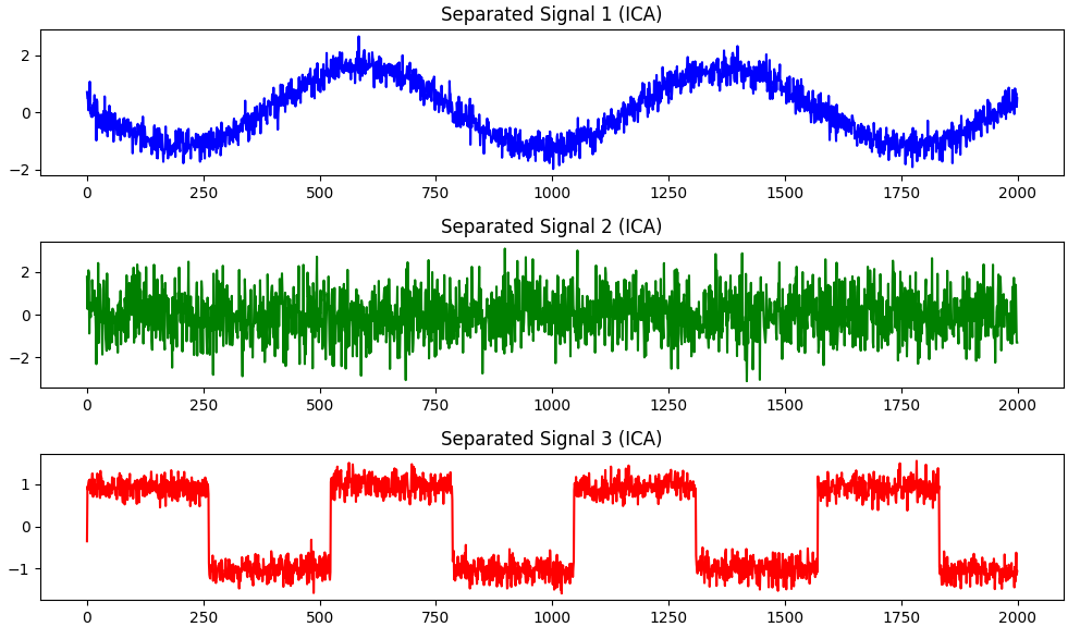
Figure 3911b shows generated synthetic mixed signals, and then ICA is used to separate them into their independent components. In this example, we generate three synthetic source signals (s1, s2, s3) and mix them using a predefined mixing matrix (A) to create mixed signals (X) with added noise. Then, we apply FastICA from scikit-learn to separate the mixed signals into their independent components (S_). Here, matplotlib is used to separate the signals. Note that ICA is a technique used in signal processing and data analysis, rather than a machine learning algorithm.    
         
         

In ICA, the scenario where there are more sources (speakers) than observed signals (microphones) is commonly referred to as an "overdetermined" or "undercomplete" case. In other words, the number of independent sources n is greater than the number of observed signals m. This is a research problem.

In an overdetermined ICA scenario:

1. Existence of Solutions:

   • The overdetermined case does not necessarily lead to a unique solution for the demixing matrix W.
   • There are multiple demixing matrices that can produce the same set of observed signals from the independent sources.
2. Source Separation Challenges:
   • The overdetermined case introduces ambiguity, and it may not be possible to uniquely determine the original sources.
   • Different demixing matrices may lead to different estimates of the sources, and these estimates might be subject to scaling and permutation ambiguities.
3. Statistical Independence:
   • While ICA aims to find statistically independent sources, the overdetermined case introduces more challenges in achieving a unique decomposition, particularly in the presence of noise or non-Gaussianity.
4. Use of Additional Information:
   • Additional information, such as knowledge about the sources or constraints on the mixing process, may be necessary to guide the ICA algorithm and obtain a meaningful solution.
5. Blind Source Separation Performance:
   • Blind source separation performance may be more challenging in the overdetermined case compared to the well-determined case (where m = n or m > n).

When there are fewer independent sources (speakers) than observed signals (microphones) in Independent Component Analysis (ICA), this scenario is commonly referred to as an "underdetermined" case. In other words, the number of independent sources n is less than the number of observed signals m. In this situation, the underdetermined ICA case presents certain challenges and considerations:

1. Existence of Solutions:

   • In the underdetermined case, there are typically multiple solutions for the demixing matrix W that can produce the same set of observed signals.
   • The sources cannot be uniquely determined from the observed signals alone.
2. Uniqueness and Ambiguity:
   • The underdetermined case introduces ambiguity, and the estimated sources may not be unique.
   • The sources can be scaled and permuted in various ways, and different demixing matrices may lead to equivalent representations of the sources.
3. Blind Source Separation Challenges:
   • Blind source separation in the underdetermined case is inherently more challenging compared to the overdetermined or well-determined cases.
   • The lack of sufficient constraints makes it difficult to uniquely identify the original sources.
4. Use of Additional Information:
   • In practice, additional information or constraints may be required to guide the ICA algorithm and improve the quality of the estimated sources.
   • Incorporating prior knowledge about the sources or the mixing process can be valuable.
5. Statistical Independence:
   • Achieving statistical independence among the estimated sources becomes more challenging in the underdetermined case.
6. Regularization Techniques:
   • Regularization techniques or additional constraints on the solution may be employed to encourage certain properties of the estimated sources, such as sparsity or smoothness.

On the other hand, determining the number of speakers (sources) in a given audio signal is a common challenge in various signal processing applications, including ICA or blind source separation. Several methods can be employed to estimate the number of speakers:

1. Spectral Analysis:

   • Use spectral analysis techniques, such as Fourier analysis, to examine the frequency content of the audio signal.
   • Apply techniques like clustering or peak detection in the frequency domain to identify distinct sources.
2. Spatial Clustering:
   • If the audio signals are recorded using multiple microphones (sensor array), exploit the spatial information.
   • Techniques like beamforming or spatial clustering can help identify distinct sound sources based on their spatial characteristics.
3. ICA with Model Order Selection:
   • Apply ICA algorithms with model order selection techniques.
   • Techniques such as information criteria (e.g., AIC or BIC) or cross-validation can help determine the optimal number of sources.
4. Source Counting Algorithms:
   • Utilize algorithms specifically designed for source counting in audio signals.
   • These algorithms often involve analyzing statistical properties of the signals to identify the number of underlying sources.
5. Non-Negative Matrix Factorization (NMF):
   • Apply NMF techniques, which decompose the observed signal into a product of non-negative matrices.
   • The resulting components can be analyzed to estimate the number of speakers.
6. Machine Learning Approaches:
   • Train machine learning models (e.g., classifiers or neural networks) to distinguish between different speakers.
   • Supervised learning methods can be employed if labeled data are available.
7. Bayesian Methods:
   • Bayesian approaches can be used to model the uncertainty in the number of sources.
   • Bayesian model selection techniques can help identify the most likely number of sources.
8. Energy-Based Methods:
   • Analyze the energy distribution in the signal to identify segments dominated by specific sources.
   • Techniques such as energy thresholding can be applied.

============================================