Posterior probability and prior probability

Posterior Probability versus Prior Probability
- Python and Machine Learning for Integrated Circuits -
- An Online Book -

Python and Machine Learning for Integrated Circuits http://www.globalsino.com/ICs/

Chapter/Index: Introduction | A | B | C | D | E | F | G | H | I | J | K | L | M | N | O | P | Q | R | S | T | U | V | W | X | Y | Z | Appendix

=================================================================================

Posterior probability and prior probability are fundamental concepts in probability theory and Bayesian statistics. Table 3836 lists the comparison between posterior probability and prior probability.

Table 3836. Posterior probability and prior probability.

	Prior probability	Posterior Probability
Definition	Prior probability represents the initial belief or probability of an event occurring before considering any new evidence or data. It is based on prior knowledge, experience, or assumptions.	Posterior probability, on the other hand, represents the updated probability of an event occurring after considering new evidence or data. It takes into account both prior beliefs and the likelihood of the evidence given those beliefs.
Notation	It is denoted as , where represents the event or hypothesis for which you want to determine the probability.	It is denoted as , where is the event or hypothesis, and is the evidence or data that has been observed.
Relationship	For instance, for Bayes' theorem, the posterior probability is calculated using Bayes' theorem, which combines the prior probability and the likelihood of the evidence: The prior probability serves as your initial belief, and the likelihood represents the probability of observing the evidence X given that P is true. The denominator is the probability of observing the evidence without any assumption about P. It is often used as a normalization factor.
Role in Bayesian Inference	It reflects your initial assumptions or beliefs about the likelihood of an event. In Bayesian inference, you start with a prior probability distribution and update it with new evidence to obtain the posterior probability distribution.	It represents the probability distribution that has been updated with new data. It is the result of Bayesian inference and provides a more informed estimate of the event's probability.
Example	Consider a medical test for a rare disease. Before any test results, you might have a prior belief that a person has a 1% chance of having the disease based on population statistics.	After conducting the test and observing the results, the posterior probability is updated based on the test's accuracy and the specific test results. This updated probability reflects the likelihood that the person has the disease given the test results.

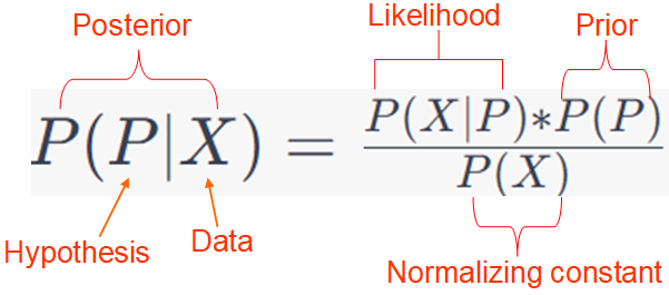
For instance, when working with probabilistic models or Bayesian classifiers, Bayes' theorem below is used for making predictions in binary classification,

-------------------------------- [3836a]

where,:

p(y=1|x) is the conditional probability that the example belongs to class 1 given the observed features x. This is the probability you want to estimate.
p(x|y=1) is the probability distribution of the features x given that the example belongs to class 1. It represents the likelihood of observing the features x when the class is 1.
p(y=1) is the prior probability of the example belonging to class 1. It represents the prior belief or probability that class 1 is the correct class.
p(x|y=0) is the probability distribution of the features x given that the example belongs to class 0 (the other class).
p(y=0) is the prior probability of the example belonging to class 0.

It is used to estimate the probability of an example belonging to a specific class, typically class 1 (y=1), based on the observed features (x).

For a specific case study, assume we're working on a binary classification problem where we want to predict whether an email is spam (class 1) or not spam (class 0) based on the presence or absence of two words: "money" and "lottery." We'll calculate the probability that an email is spam (y=1) given the observed words (x) using Equation 3836a.

Let's assume the following probabilities:

Probability that an email is spam: , which is the prior probability. It represents the prior probability or prior belief that an email is spam (class 1) without considering any specific observed words. It is your initial belief in the absence of evidence.
Probability that an email is not spam:

Now, let's consider the probabilities of observing the words "money" and "lottery" in both spam and non-spam emails:

Probability of observing "money" in a spam email:
Probability of observing "money" in a non-spam email:
Probability of observing "lottery" in a spam email:
Probability of observing "lottery" in a non-spam email:

Now, suppose you receive an email that contains both "money" and "lottery" (x = ["money", "lottery"]). You want to determine whether this email is spam (y=1) or not (y=0).

Using Equation 3836a, substituting the probabilities:

-------------------------------- [3836b]

Then, the posterior probability p(y=1|x), which represents the probability that the email is spam (class 1) given the observed words "money" and "lottery.", is equal to 6. Therefore, the probability that this email is spam (y=1) given the words "money" and "lottery" is 6 times higher than it being not spam (y=0). In this case, you would predict that the email is likely spam. This is a simplified example, but it demonstrates how the formula can be used to calculate class probabilities in a binary classification scenario.

In this example above, p(y =1|x) is the probability you want to compute after considering the evidence (the words "money" and "lottery"), while p(y=1) is your initial belief about the probability of an email being spam.

In Bayesian statistics, the equation on the updated probability distribution of parameters or hypotheses, which represents the updated probability distribution of parameters or hypotheses based on observed data, can be given by,

P(θ|D) ∝ P(D|θ) * P(θ) ---------------------------------- [3836c]

where:

P(θ|D) is the posterior distribution of the parameter θ given data D.
P(D|θ) is the likelihood of observing data D given parameter θ.
P(θ) is the prior distribution of the parameter θ.
∝ denotes proportionality, indicating that the right-hand side is proportional to the left-hand side.

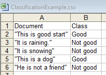
Next example is to find which class, for a document, maximize the posterior possibility with Bayes' Theorem:

------------------------ [3836d]

-------------- [3836e]

--- [3836f]

--------------------------- [3836g]

where,

word₁, word₂, word₃, ..., word_n are the words in the particular document.

If there are too many words in the documents, then we can make two assumptions:

i) Word order does not matter, so we use BOW representations.

ii) Word appearances are independent of each other given a particular class. This is why "Naive" comes from. However, in real life, some words, e.g. "Thank" and "you" are correlated.

The Naive Bayes Classifier is given by the log formula below,

--------------------------- [3836h]

For instance, a csv file has contents below:

Then, the Priors, P(c) are:

P(Good) = 2/5

P(Not good) = 3/5

============================================

=================================================================================