=================================================================================
Naive Bayes is a generative model because it uses knowledge about the underlying probability distributions that generate the data being analyzed. It's capable of generating new data points. Text classification, also known as document classification or supervised text categorization, involves assigning predefined labels or categories to text documents based on their content. The goal is to train a model to recognize patterns and associations between the content of documents and the appropriate labels. To do this, you need a labeled dataset where each document is associated with its correct category or label.
Key Points:
- Supervised learning: Requires labeled training data.
- Documents are assigned to specific predefined categories.
- Ground truth labels are needed for training and evaluation.
- Common algorithms include Naive Bayes [1-9], Support Vector Machines (SVM), and deep learning approaches like Convolutional Neural Networks (CNN) and Recurrent Neural Networks (RNN).
- Example use case: Categorizing emails as spam or not spam.
Naive Bayes is a probabilistic classification, supervised machine learning algorithm commonly used for classification and probabilistic modeling. It's based on Bayes' theorem, which is a fundamental concept in probability theory. Naive Bayes is particularly popular for text classification tasks, such as spam email detection and sentiment analysis, although it can be applied to other types of data as well.
In a supervised setting, the Naive Bayes algorithm requires labeled training data, where each data point is associated with a class label. The algorithm learns the conditional probability of a particular class given a set of features or attributes. Despite its "naive" assumption that features are conditionally independent (which might not always hold in real-world scenarios), Naive Bayes often performs surprisingly well and is computationally efficient.
Naive Bayes is a probabilistic machine learning algorithm that's used for classification tasks. Unlike some other algorithms such as linear regression or support vector machines, Naive Bayes does not explicitly use feature weights in the same way. Instead, it relies on probabilities and conditional probabilities to make predictions.
Text classification with Naive Bayes offers several advantages, making it a popular choice for various natural language processing tasks:
-
Simplicity and Efficiency: Naive Bayes is relatively simple to understand and implement. It doesn't require complex parameter tuning, and its computational efficiency makes it well-suited for large datasets.
-
Scalability: Naive Bayes can handle a large number of features (words) with ease, making it suitable for high-dimensional data such as text.
-
Quick Training: Training a Naive Bayes classifier is often fast, especially compared to more complex algorithms like deep learning models.
-
Small Amount of Data: Naive Bayes can perform well even when the amount of training data is small. This is particularly useful in scenarios where you don't have a vast amount of labeled examples.
-
Interpretability: The probabilistic nature of Naive Bayes allows for easy interpretation of results. You can understand why a certain classification decision was made based on the calculated probabilities.
-
Low Overfitting Risk: Naive Bayes has a lower risk of overfitting compared to more complex algorithms. Its simplifying assumptions (naive independence) can act as a form of regularization.
-
Good Baseline: Naive Bayes often serves as a solid baseline model. If it performs well on a specific problem, you might not need to explore more complex models.
-
Real-time Applications: Due to its speed and efficiency, Naive Bayes can be used in real-time applications where quick decisions are required.
-
Textual Data Handling: Naive Bayes handles textual data well, and it's particularly suited for text classification tasks such as sentiment analysis, spam detection, topic categorization, and more.
-
Incremental Learning: Naive Bayes supports incremental learning, where the model can be updated with new data without needing to retrain from scratch. This is useful for scenarios where new data arrives over time.
It's important to note that while Naive Bayes has these advantages, it might not always be the best choice for every text classification problem. Its assumption of feature independence might not hold true in all cases, and more complex models like deep learning methods might be necessary for certain tasks where capturing intricate relationships in the data is crucial.
While Naive Bayes has several advantages for text classification, it also has some limitations and disadvantages:
-
Assumption of Feature Independence: The "naive" assumption of feature independence might not hold true for all types of text data. In natural language, words often have contextual relationships, and this assumption can lead to suboptimal performance in some cases.
-
Lack of Contextual Information: Naive Bayes doesn't take into account the order or context of words in a document. This can be a significant limitation for tasks that require understanding the sequential or contextual nature of text, such as language modeling or certain types of sentiment analysis.
-
Handling Out-of-Vocabulary Words: Naive Bayes struggles with out-of-vocabulary words or words that were not seen during training. Since it relies on calculating probabilities based on the training data, encountering unseen words can lead to inaccurate classifications.
-
Limited Expressiveness: Due to its simplicity, Naive Bayes may not capture complex patterns in the data as well as more advanced algorithms like deep learning models. It might struggle with tasks that require learning intricate relationships between features.
-
Sensitive to Data Quality: Naive Bayes is sensitive to the quality of the training data. If the training data contains noise, irrelevant features, or mislabeled examples, it can negatively impact the model's performance.
-
Imbalanced Data: When dealing with imbalanced classes, Naive Bayes can be biased toward the majority class. This is because it estimates probabilities based on the class distribution in the training data.
-
Limited Performance on Highly Complex Tasks: While Naive Bayes can serve as a strong baseline, it might not achieve state-of-the-art performance on extremely complex tasks where deep learning or more advanced models are better suited.
-
Difficulty with Continuous Features: Naive Bayes works best with discrete features (like word counts). It may struggle to handle continuous features effectively without discretization.
-
Sensitive to Feature Variations: Small changes or variations in the input features can disproportionately affect Naive Bayes' predictions. This can make the model less robust in noisy environments.
-
Not Always the Best Probabilistic Estimator: While Naive Bayes is based on Bayesian principles, it might not always produce well-calibrated probability estimates, which could be important in certain applications.
-
Inability to Handle Complex Relationships: It cannot capture complex relationships between features, which can be a limitation for tasks that require understanding nuanced connections between words.
Despite these disadvantages, Naive Bayes remains a valuable tool in the field of text classification, especially for simpler tasks or as a baseline comparison against more advanced techniques. It's important to carefully consider the characteristics of your data and the requirements of your task before deciding whether Naive Bayes is the appropriate choice.
In the field of natural language processing and text analysis, researchers and practitioners often conduct report analyses to evaluate the performance of various algorithms, including Naive Bayes, on different text classification tasks. These reports can encompass a wide range of applications and domains, such as sentiment analysis, spam detection, topic categorization, document classification, and more.
Here's what you might typically find in a report analysis related to text classification with Naive Bayes:
-
Problem Statement: A clear description of the text classification task being addressed, such as sentiment analysis of social media posts, categorization of news articles, etc.
-
Dataset Description: Details about the dataset used for training and testing the Naive Bayes classifier. This includes information about the size of the dataset, class distribution, and any preprocessing steps applied to the text data.
-
Experimental Setup: Information about how the experiments were conducted, including how the dataset was split into training and testing sets, any cross-validation procedures, and parameter settings for the Naive Bayes algorithm.
-
Performance Metrics: Evaluation metrics used to assess the performance of the Naive Bayes classifier, such as accuracy, precision, recall, F1-score, and possibly area under the ROC curve (AUC).
-
Baseline Comparisons: Comparison of Naive Bayes performance with other classification algorithms or approaches. This could include traditional machine learning algorithms as well as more advanced techniques like deep learning models.
-
Results and Analysis: Presentation of the classification results, possibly in the form of confusion matrices, ROC curves, precision-recall curves, and discussions of the model's strengths and weaknesses.
-
Discussion of Findings: Interpretation of the results, identification of challenges faced during the classification task, and insights gained from the analysis.
-
Related Work: A review of relevant literature and existing approaches to text classification, including discussions of how Naive Bayes compares to other methods.
-
Conclusion: A summary of the findings, implications of the results, and potential directions for future research or improvements.
To find specific report analyses related to text classification with Naive Bayes, you can search academic databases (such as IEEE Xplore, ACM Digital Library, or Google Scholar) using relevant keywords and filters like publication date. Remember that the availability of such reports may vary, and it's always a good idea to ensure that the information is current and relevant to your specific interests.
In the semiconductor industry, failure analysis involves identifying and understanding the reasons behind defects or failures in semiconductor devices or processes. Text classification, in combination with techniques from natural language processing (NLP), could aid in automating parts of the failure analysis process by analyzing textual reports, logs, and documentation associated with semiconductor manufacturing and testing. The outline below shows how text classification using Naive Bayes might be applied to failure analysis in the semiconductor industry:
-
Data Collection and Preprocessing: Gather textual data sources relevant to semiconductor failure analysis, such as test reports, equipment logs, maintenance notes, defect descriptions, and customer feedback. Preprocess the text data by removing noise, standardizing terms, and tokenizing the text into features.
-
Labeling and Categorization: Manually label or categorize the text data based on different failure modes, defect types, process issues, or other relevant categories. This labeled data will be used for training and evaluating the Naive Bayes classifier.
-
Feature Extraction: Convert the textual data into numerical features that Naive Bayes can work with. Common techniques include bag-of-words representation, TF-IDF (Term Frequency-Inverse Document Frequency) weighting, and word embeddings.
-
Training the Naive Bayes Classifier: Train a Naive Bayes classifier on the labeled data. The classifier learns the relationships between the extracted features and the predefined failure categories.
-
Model Evaluation: Evaluate the performance of the Naive Bayes classifier using appropriate metrics such as accuracy, precision, recall, and F1-score. Cross-validation and parameter tuning can be used to optimize the model's performance.
-
Failure Mode Prediction: Once the Naive Bayes classifier is trained, it can be used to automatically predict or categorize failure modes based on new, unlabeled textual data. For example, it could analyze incoming defect reports and provide insights into potential failure causes.
-
Error Analysis and Interpretability: Analyze misclassified instances to understand potential limitations and areas for improvement. Explore techniques to interpret the model's decisions, such as feature importance or explanation methods.
-
Continuous Improvement: Refine the classifier over time by incorporating new labeled data and iteratively improving its performance.
While Naive Bayes can be a useful tool for certain aspects of failure analysis in the semiconductor industry, it's important to acknowledge its limitations, especially the assumption of feature independence. For more complex relationships and nuanced analyses, more advanced machine learning approaches or hybrid methods might be needed.
To find specific report analyses related to Naive Bayes and failure analysis in the semiconductor industry, you may need to search specialized industry publications, conference proceedings, or research databases with a focus on semiconductor manufacturing, reliability, and failure analysis.
When using Naive Bayes for text classification, there are several important considerations and tricks that can help improve the performance and effectiveness of your model. Here are some key tricks to keep in mind:
-
Feature Engineering:
- Text Preprocessing: Clean and preprocess your text data by removing punctuation, converting to lowercase, and handling special characters.
- Tokenization: Split text into individual words or tokens.
- Stop Words Removal: Remove common words that don't provide significant meaning.
- Stemming and Lemmatization: Reduce words to their root form to avoid duplication of similar words.
- N-grams: Consider using bi-grams or tri-grams to capture context between adjacent words.
- Feature Representation:
- Bag-of-Words (BoW): Represent text as a vector of word frequencies in the document.
- TF-IDF (Term Frequency-Inverse Document Frequency): Assign weights to words based on their importance in the corpus.
- Word Embeddings: Utilize pre-trained word embeddings like Word2Vec, GloVe, or FastText to capture semantic relationships.
- Handling Rare Words and Outliers:
- Set a threshold for word frequency to exclude rare words that might introduce noise.
- Consider handling spelling errors and typos using techniques like Levenshtein distance.
- Model Selection:
- Multinomial Naive Bayes: Commonly used for text classification tasks.
- Gaussian Naive Bayes: Applicable when feature values follow a Gaussian distribution.
- Complement Naive Bayes: Designed to address imbalanced class distribution.
- Smoothing:
- Apply Laplace (additive) smoothing to handle zero probabilities and prevent overfitting. However, Naive Bayes algorithm is generally not sensitive to zero values in the features under the assumption of feature independence (see page3675).
- Class Imbalance:
- Address class imbalance using techniques like oversampling, undersampling, or using specialized Naive Bayes variants like ComplementNB.
- Parameter Tuning:
- Experiment with hyperparameters such as alpha (smoothing parameter) to optimize model performance.
- Ensemble Methods:
- Combine multiple Naive Bayes models or other classifiers through techniques like bagging or boosting.
- Text Length:
- Normalize text length by using fixed-length features (e.g., BoW, TF-IDF) to ensure consistent input dimensions.
- Evaluation and Validation:
- Use appropriate evaluation metrics (accuracy, precision, recall, F1-score) based on the nature of your text classification problem.
- Perform cross-validation to assess model performance on different data subsets.
- Handling Out-of-Vocabulary Words:
- Consider using sub-word embeddings or character-level models to handle out-of-vocabulary words.
- Domain-Specific Knowledge:
- Incorporate domain-specific knowledge or domain-specific word lists if available.
- Regularization:
- Use L1 or L2 regularization to prevent overfitting and improve model generalization.
- Model Interpretability:
- Naive Bayes models provide interpretable results in terms of feature probabilities, which can be useful for understanding model decisions.
- Pipeline and Workflow:
- Create a well-structured pipeline for data preprocessing, feature extraction, modeling, and evaluation.
Note that while Naive Bayes is a simple and effective algorithm for text classification, its "naive" assumption of feature independence may not always hold true for complex language patterns. Therefore, it's important to combine these tricks with a thorough understanding of your specific text classification problem and dataset to achieve optimal results.
Naive Bayes uses likelihood and prior probability to calculate the conditional probability of the class. The likelihood component in Naive Bayes refers to the probability of observing a particular set of feature values given the class. It essentially quantifies how likely it is to see the given features if the class is known. In a Naive Bayes classifier, the likelihood represents the probability of observing a particular feature (or word) given a specific class label. In other words, it calculates the probability that a certain feature would appear in a document of a particular class. This likelihood estimation is a crucial part of the Naive Bayes algorithm. The prior probability represents the probability of each class occurring independently, without considering any specific features. In a classification problem, it is important to know the prior probability of each class in the absence of any evidence from the features.
Here's how the likelihood is calculated in the context of a text classification problem using a Naive Bayes classifier:
-
Feature Extraction: The input text documents are transformed into a set of features (words or tokens) using techniques like CountVectorizer or TF-IDF (Term Frequency-Inverse Document Frequency).
-
Calculating Likelihood: For each class label in your classification problem, the likelihood of a feature given that class is calculated. This is usually done using the frequency of the feature in documents of that class. For example, if you have a class "spam" and a feature "free," you would calculate the likelihood of "free" occurring in "spam" emails.
-
Naive Assumption: The "naive" assumption in Naive Bayes is that the features are conditionally independent given the class label. This means that the presence of one feature doesn't affect the presence of another feature in the same class. This assumption simplifies the calculations by assuming that each feature's contribution to the probability can be considered independently.
-
Bayes' Theorem: The likelihood, along with the prior probability of each class and the probability of the features given any class, is used in Bayes' theorem to calculate the posterior probability of each class given the observed features. The class with the highest posterior probability is predicted as the final class label.
To summarize, the likelihood in Naive Bayes represents the conditional probability of observing a specific feature given a class label. It is used in conjunction with other probabilities and the Naive Bayes formula to classify new instances. As an example, Figure 4026a shows the probabilities like Overcast probability = 0.29 and probability of playing is 0.64.
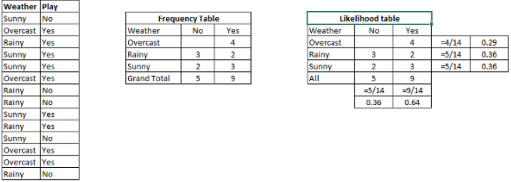
Figure 4026a. Creating Likelihood table by finding the probabilities. [10]
In the code above, pipelines are not explicitly used. However, the code demonstrates the concept of a machine learning pipeline, even though it's implemented in a manual step-by-step manner:
-
Import Libraries: The necessary libraries like pandas, CountVectorizer from sklearn.feature_extraction.text, and MultinomialNB from sklearn.naive_bayes are imported.
-
Reading Data: The code reads data from a CSV file into a pandas DataFrame. This data is presumably used for training and prediction.
-
Extracting Training Data: The training data (features and labels) are extracted from the DataFrame. X_train contains the text data from 'ColumnA' excluding the header, and y_train contains the corresponding labels from 'ColumnB'.
-
Preprocessing Training Data: The training text data is preprocessed using the CountVectorizer. This step involves tokenizing the text data, converting it into a bag-of-words representation, and creating a sparse matrix X_train_vec that represents the features.
-
Training a Classifier: A Multinomial Naive Bayes classifier (clf) is initialized and trained using the bag-of-words features (X_train_vec) and the corresponding labels (y_train).
-
New String for Prediction: A new string (MyNewString) is created for which a prediction needs to be made.
-
Preprocessing New String: The new string is preprocessed in the same way as the training data using the same CountVectorizer. The result is a sparse matrix new_string_vec representing the new string in the same format as the training data.
-
Predicting with Classifier: The trained classifier is then used to predict the label for the new string by applying it to the preprocessed features of the new string. The predicted label is stored in predicted_value.
-
Printing Prediction: The predicted label is printed to the console.
A machine learning pipeline typically includes multiple sequential steps, such as data preprocessing, feature extraction, model training, and prediction. These steps are encapsulated within a pipeline object, which makes it easier to manage and automate the entire process. Pipelines also provide mechanisms for hyperparameter tuning and cross-validation.
In the given code above, while the steps are implemented manually, they do align with the general idea of a machine learning pipeline, where data is processed, transformed, and used to train and make predictions with a model. Using an actual pipeline can make the code more modular, readable, and easier to maintain.
The part of the code, above, that indicates the Naive Bayes Classifier and demonstrates how it works is as follows:
# Train a Naive Bayes classifier
clf = MultinomialNB()
clf.fit(X_train_vec, y_train)
Here's what this part of the code does:
-
Initialization: A new instance of the MultinomialNB class, which represents a Multinomial Naive Bayes classifier, is created and stored in the variable clf.
-
Training: The fit method is called on the classifier (clf). This method takes the training features (X_train_vec) and corresponding labels (y_train) as arguments. The classifier uses this data to learn the statistical patterns in the text data and build a model that can predict the labels based on the given features.
The Naive Bayes classifier is a probabilistic machine learning model that is based on the Bayes' theorem. In the case of the Multinomial Naive Bayes classifier, it's specifically designed for working with text data where the features represent word counts or frequencies. The "naive" assumption in Naive Bayes refers to the assumption that the features (words in this case) are conditionally independent given the class label. This assumption simplifies the calculations and makes the model computationally efficient.
The classifier calculates the probabilities of a given input (a set of words) belonging to each possible class label. It does this by utilizing the Bayes' theorem and by assuming the independence of the features. The class with the highest calculated probability is then predicted as the label for the input.
After the training process, the classifier is ready to make predictions. In your code, the trained classifier (clf) is used to predict the label for a new string (MyNewString) using the predict method. The preprocessed features of the new string (new_string_vec) are provided as input, and the predicted label is obtained. This label is then printed to the console.
Naive Bayes classifier can be used to work on both binary classification and multi-class classification problems:
1. Binary Classification:
In binary classification, you have two classes (e.g. shown in Table 4026a), typically denoted as "positive" (P) and "negative" (N). Given a set of features (X), you want to determine the probability that an observation belongs to the positive class.
The probability of an observation belonging to the positive class, given the features, is calculated using Bayes' theorem as follows:
 ------------------------------------------ [4026a] ------------------------------------------ [4026a]
Where:
- P(P|X) is the posterior probability that the observation belongs to the positive class.
- P(X|P) is the likelihood of observing the features X given that the class is positive.
- P(P) is the prior probability of the positive class.
- P(X) is the probability of observing the features X.
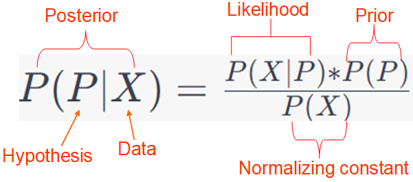
Table 4026a. Binary classification.

2. Multi-Class Classification:
In multi-class classification, you have more than two classes (e.g. shown in Table 4026b), typically denoted as C1, C2, … , Ck, where k is the number of classes. Given a set of features (X), you want to determine the probability that an observation belongs to each class.
The probability of an observation belonging to class Ci (where i varies from 1 to k), given the features, is calculated using Bayes' theorem as follows:
 ------------------------------------------ [4026b] ------------------------------------------ [4026b]
Where:
- P(Ci|X) is the posterior probability that the observation belongs to class Ci.
- P(X|Ci) is the likelihood of observing the features X given that the class is Ci.
- P(Ci) is the prior probability of class Ci.
- The denominator is the sum of the probabilities for all classes and serves as a normalization factor to ensure that the probabilities sum to 1.
Table 4026b. Multi-class classification.

"X" in the Naive Bayes classification and many other machine learning algorithms often represents the feature vector. A feature vector is a numerical representation of the features or attributes of a data point. Each component or element of the feature vector corresponds to a specific feature, and together they provide a concise and structured representation of the data for the algorithm to work with. Both Multinomial Naive Bayes and the standard (single) Naive Bayes algorithm can work with feature vectors. In single Naive Bayes classification for text, word frequencies, presence or absence of specific words, and other relevant properties of the text are used to create feature vectors. These feature vectors are numerical representations of the text data that the Naive Bayes algorithm uses for classification. This approach represents the document as a binary feature vector. Each element in the vector corresponds to the presence (1) or absence (0) of a particular word in the document:
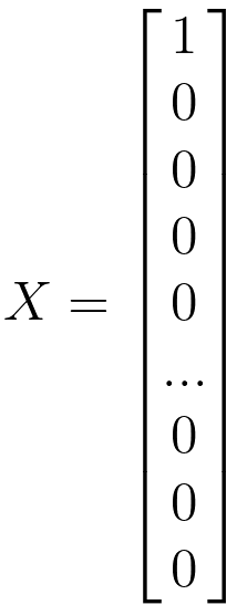 ------------------------------------------------------- [4026c] ------------------------------------------------------- [4026c]
 ------------------------------------------------------- [4026d] ------------------------------------------------------- [4026d]
Each element in this vector in Equation 4026c represents the value of a specific feature. For instance, word Xi indicates {word i appears in an document}. There are 2n possible vectors of Xi, there are then 2n parameters.
Assuming Xi's are conditionally independent given y, then we have,
p(X1, X2, ..., Xn) = p(X1|y)p(X2|X1, y) p(X3|X1, X2, y) ... p(Xn|X1, X2, ... Xn-1, y) ----------------------------- [4026e]
We can assume,
p(X1, X2, ..., Xn) = p(X1|y) p(X2|y) p(X3|y) ... p(Xn|y)----------------------------- [4026f]
Then, the joint probability distribution of n random variables x1, x2, ..., xn, conditioned on the variable y can be given by,
 ------------------------------------------ [4026g] ------------------------------------------ [4026g]
Equation 4026f simplifies the calculation of likelihood by assuming conditional independence among input parameters, which is called conditional independence assumption or Naive Bayes assumption. This is not true mathematical assumption, but it is not so horrible in practice.
The parameters in the model are:
Φj|y=1 = p(xj = 1|y = 1) ------------------------------------ [4026h]
Φj|y=0 = p(xj = 1|y = 0) ------------------------------------ [4026i]
Φy = p(y=1) ------------------------------------ [4026j]
Therefore, to build the generative model, we need to model p(x|y) and p(y).
By using joint likelihood,
 -------------------------------- [4026k] -------------------------------- [4026k]
We can find the maximum likelihood estimation given by,
 -------------------------------- [4026l] -------------------------------- [4026l]
 -------------------------------- [4026m] -------------------------------- [4026m]
where,
 is a notation of an indicator function or characteristic function, which is commonly used in statistics and mathematics to represent a function that takes on the value 1 when a particular condition is met and 0 otherwise: is a notation of an indicator function or characteristic function, which is commonly used in statistics and mathematics to represent a function that takes on the value 1 when a particular condition is met and 0 otherwise:
- It equals 1 when both conditions are satisfied: xj(i) = 1 and y(i) = 1 for the ith observation in the dataset.
- It equals 0 when either xj(i) = 1 or y(i) is not 1 for the ith observation.
The use of this indicator function allows you to count the number of times both conditions are met, which can be useful when calculating conditional probabilities shown in Equation 4026m. The numerator counts how many times both xj and y are 1 for the ith observation, and the denominator counts how many times y is 1 in the dataset.
Then, when working with probabilistic models or Bayesian classifiers, Bayes' theorem below is used for making predictions in binary classification,
 -------------------------------- [4026n] -------------------------------- [4026n]
where,:
-
p(y=1|x) is the conditional probability that the example belongs to class 1 given the observed features x. This is the probability you want to estimate.
-
p(x|y=1) is the probability distribution of the features x given that the example belongs to class 1. It represents the likelihood of observing the features x when the class is 1.
-
p(y=1) is the prior probability of the example belonging to class 1. It represents the prior belief or probability that class 1 is the correct class.
-
p(x|y=0) is the probability distribution of the features x given that the example belongs to class 0 (the other class).
-
p(y=0) is the prior probability of the example belonging to class 0.
It is used to estimate the probability of an example belonging to a specific class, typically class 1 (y=1), based on the observed features (x).
For a specific case study, assume we're working on a binary classification problem where we want to predict whether an email is spam (class 1) or not spam (class 0) based on the presence or absence of two words: "money" and "lottery." We'll calculate the probability that an email is spam (y=1) given the observed words (x) using Equation 4026n.
Let's assume the following probabilities:
- Probability that an email is spam: p(y = 1) = 0.4, which is the prior probability. It represents the prior probability or prior belief that an email is spam (class 1) without considering any specific observed words. It is your initial belief in the absence of evidence.
- Probability that an email is not spam: p(y = 0) = 0.6
Now, let's consider the probabilities of observing the words "money" and "lottery" in both spam and non-spam emails:
- Probability of observing "money" in a spam email: p("money"|y = 1) = 0.9
- Probability of observing "money" in a non-spam email: p("money"|y = 0) = 0.1
- Probability of observing "lottery" in a spam email: p("lottery"|y = 1) = 0.8
- Probability of observing "lottery" in a non-spam email: p("lottery"|y = 0) = 0.2
Now, suppose you receive an email that contains both "money" and "lottery" (x = ["money", "lottery"]). You want to determine whether this email is spam (y=1) or not (y=0).
Using Equation 4026n, substituting the probabilities:
 -------------------------------- [4026o] -------------------------------- [4026o]
Then, the posterior probability p(y=1|x), which represents the probability that the email is spam (class 1) given the observed words "money" and "lottery.", is equal to 6. Therefore, the probability that this email is spam (y=1) given the words "money" and "lottery" is 6 times higher than it being not spam (y=0). In this case, you would predict that the email is likely spam. This is a simplified example, but it demonstrates how the formula can be used to calculate class probabilities in a binary classification scenario.
In this example above, p(y =1|x) is the probability you want to compute after considering the evidence (the words "money" and "lottery"), while
p(y=1) is your initial belief about the probability of an email being spam.
Note that adding 1 to the numerator and 2 to the denominator is a technique used to handle cases where you have very limited data and want to avoid division by zero or extreme probabilities in a Bayesian setting. This is known as Laplace smoothing, Laplace correction, or add-one smoothing, and it's commonly used when dealing with small sample sizes in probability calculations. The idea behind Laplace smoothing is to provide a small, non-zero probability estimate for events that have not been observed in the data. This is particularly useful in Bayesian statistics and probabilistic models to avoid situations where you have zero counts in your data, which can lead to problematic calculations. In this case, Equation 4026n becomes,
 -------------------------- [4026p] -------------------------- [4026p]
TF-IDF is a more advanced way to create feature vectors for text data. It takes into account the frequency of words in a document relative to their frequency across the entire dataset. This allows it to emphasize words that are important to a specific document while de-emphasizing common words.
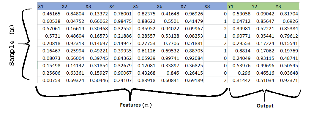
Table 4026c. Multiple training samples, features, and outputs in csv format.

The scaling of  with respect to n for the Naive Bayes algorithm can depend on several factors, including the assumptions made about the data and the model. [11,12] However, in many cases, the excess risk for the Naive Bayes algorithm tends to converge at a rate close to 1/n1/2. Here's a simplified explanation of why this might be the case: with respect to n for the Naive Bayes algorithm can depend on several factors, including the assumptions made about the data and the model. [11,12] However, in many cases, the excess risk for the Naive Bayes algorithm tends to converge at a rate close to 1/n1/2. Here's a simplified explanation of why this might be the case:
-
Naive Bayes Algorithm: The Naive Bayes algorithm is often used for classification tasks. It's based on Bayes' theorem and makes a strong independence assumption between the features. While this assumption simplifies the model and makes it computationally efficient, it may not fully capture complex relationships in the data.
- Excess Risk Convergence: The excess risk (
 ) measures the difference between the risk of the learned Naive Bayes model (ℎ^) and the risk of the best possible model (ℎ*). The rate at which this excess risk converges to zero depends on the quality of the model and the richness of the data. ) measures the difference between the risk of the learned Naive Bayes model (ℎ^) and the risk of the best possible model (ℎ*). The rate at which this excess risk converges to zero depends on the quality of the model and the richness of the data.
- Complexity: The Naive Bayes model is relatively simple, assuming independence between features. As a result, it might struggle to capture complex patterns in the data, especially when the number of features or the dimensionality of the problem is high.
- Sample Size (n): When the sample size (n) is small relative to the dimensionality of the problem, it can be challenging for the Naive Bayes algorithm to learn accurate models. In such cases, the excess risk might converge more slowly, closer to 1/n1/2, because the algorithm has limited information to generalize from.
- Noisy Data: If the data contains noise or irrelevant features, it can impact the convergence rate. The Naive Bayes algorithm might struggle to distinguish between signal and noise, leading to slower convergence.
- Assumptions: It's important to note that the exact convergence rate can vary based on specific assumptions about the data distribution and the way in which the Naive Bayes model is fit to the data.
Therefore, while the Naive Bayes algorithm is a simple and efficient classification method, its convergence rate for the excess risk  can be relatively slow, often scaling with 1/n1/2. This is because of the model's simplicity and the challenges it faces in capturing complex dependencies in the data, especially when the sample size is limited. However, the exact behavior may still depend on the specific problem and assumptions. can be relatively slow, often scaling with 1/n1/2. This is because of the model's simplicity and the challenges it faces in capturing complex dependencies in the data, especially when the sample size is limited. However, the exact behavior may still depend on the specific problem and assumptions.
Naive Bayes algorithms can employ different models for machine learning tasks, and the choice of model depends on the nature of the data and the problem you are trying to solve, for instance,
-
Multinomial Naive Bayes:
- The Multinomial Naive Bayes model is commonly used for text classification tasks, such as spam detection, sentiment analysis, and document classification.
- It is suitable when your data consists of counts or frequencies of features, like word occurrences in a document.
- It assumes that the features are generated from a multinomial distribution.
- Multivariate Bernoulli Naive Bayes:
- The Multivariate Bernoulli Naive Bayes model is used for binary data, where features are either present or absent (i.e., binary features).
- It is commonly applied in problems like image classification, where the presence or absence of certain visual features is important.
- It assumes that the features are generated from a set of independent Bernoulli distributions.
- Gaussian Naive Bayes.
- Multinomial Event Model.
- Multivariate Bernoulli Learning Model.
However, Naive Bayes algorithms in some cases are not very competitive because some reason below:
-
Simplistic Assumptions: Naive Bayes algorithms make the strong assumption that features are conditionally independent, which is often not true in real-world data. This simplification can limit their performance in cases where the relationships between features are more complex.
-
Lack of Model Capacity: Naive Bayes models are relatively simple and have a limited capacity to capture intricate patterns in data. This can lead to suboptimal performance in tasks that require more complex and nuanced modeling.
-
Performance Compared to Deep Learning: In many modern machine learning tasks, deep learning models, such as convolutional neural networks (CNNs) for image processing or recurrent neural networks (RNNs) for natural language processing, have achieved state-of-the-art results. Naive Bayes models are often not as competitive as these deep learning models on tasks where large amounts of data and complex patterns need to be captured.
-
Data Type Limitations: Naive Bayes models are well-suited for specific types of data, such as text or simple categorical data. They may not be competitive in tasks involving structured or high-dimensional data.
-
Data Preprocessing Challenges: The performance of Naive Bayes models can be sensitive to the quality of feature engineering and preprocessing. If these steps are not performed effectively, the model's performance can suffer.
============================================
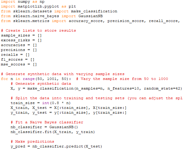
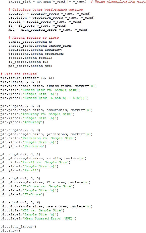
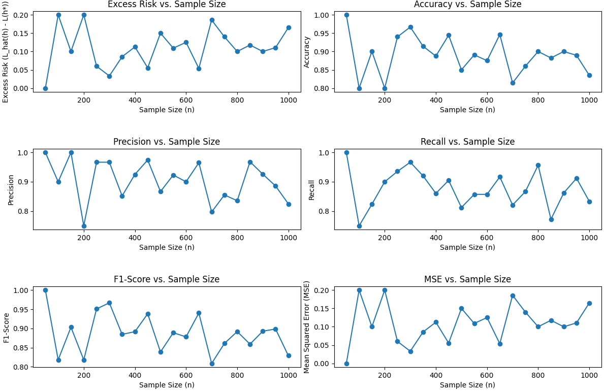
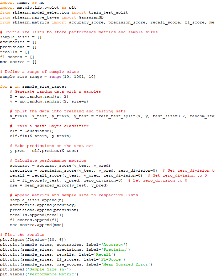
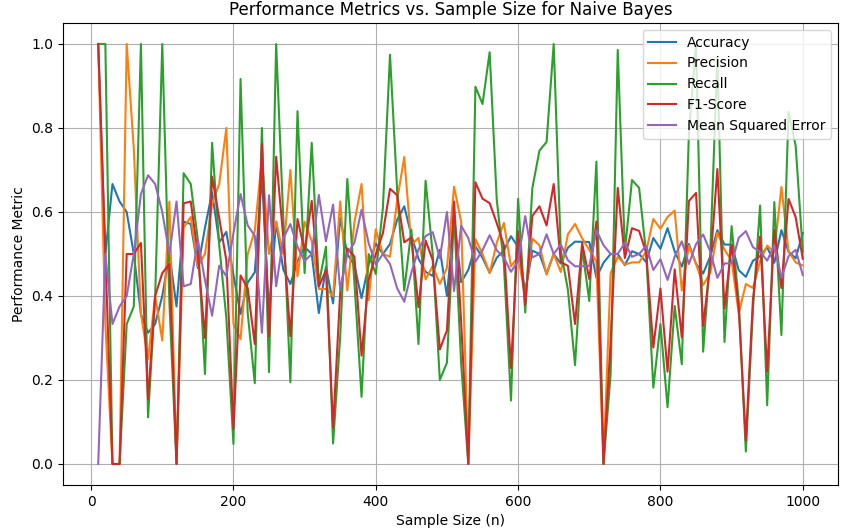
Plot the relationship betweeen  and samle size n, Accuracy, Precision, Recall, F1-Score and Mean Squared Error for Naive Bayes algorithm. Code: and samle size n, Accuracy, Precision, Recall, F1-Score and Mean Squared Error for Naive Bayes algorithm. Code:


Output:

In this script, we create synthetic data with varying sample sizes, fit a Gaussian Naive Bayes classifier, calculate various performance metrics, and then plot the relationships between these metrics and sample size.
============================================
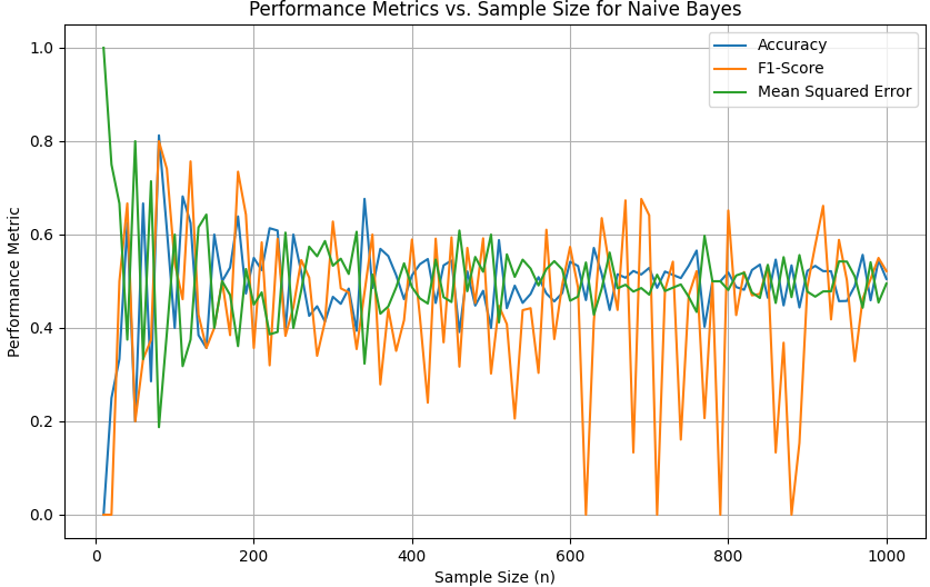
Here, we generate random data with varying sample sizes and evaluate the Naive Bayes classifier's performance metrics in order to plot the dependencies of accuracy, precision, recall, F1-Score, and Mean Squared Error (MSE) on sample size n for a Naive Bayes algorithm. Code:


Output:


An example of the procedures (or steps) of constructing a Naive Bayes Classifier for text classification are below:
-
Preprocessing and Creating a Word Dictionary: Preprocessing text data to clean and tokenize it is a crucial first step in any text classification task. Creating a dictionary of words and their counts in the training data is a common practice, as it helps in building the probability models.
-
Calculating Word Probabilities: Calculating the probability of each word in a text is part of feature engineering. Filtering out words with probabilities below a certain threshold is helpful in reducing noise in the data.
-
Creating Probability Models for Words: This step involves calculating probabilities for each word being present in both insincere and sincere questions. It's a fundamental step for building a Naive Bayes model.
-
Finding Conditional Probabilities: This refers to calculating conditional probabilities, which are essential for Naive Bayes classification. These probabilities are used in the classification process.
-
Prediction Using Conditional Probabilities: Once the conditional probabilities are established, they can be used to classify new texts into either insincere or sincere categories.
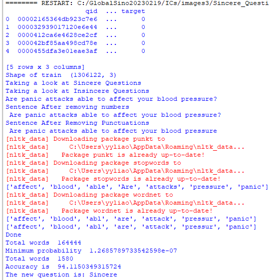
Here is the input and output of an example of classification of "Sincere Questions" and "Insincere Questions" using Naive Bayes algorithm (Code):
Input:

Output:

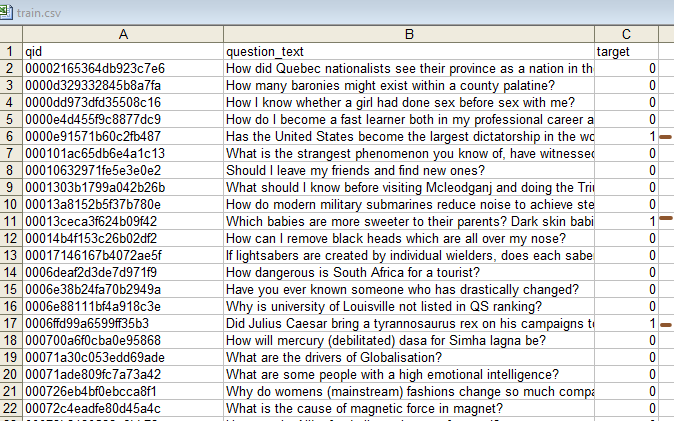
In the script above, the following columns from your "training" CSV file are used:
-
qid: The "qid" column likely contains unique identifiers (Question IDs) for each question in the dataset. This column is not explicitly mentioned in the script, but it is typically used to uniquely identify questions and is used internally or for reference.
-
question_text: The "question_text" column contains the actual text of the questions. This column is processed and used for various text preprocessing and classification tasks within the script.
-
target: The "target" column is used to determine whether a question is classified as "sincere" (0) or "insincere" (1). This column is important for training the model and evaluating its performance on the training and test datasets.
The lines in the script that use the "target" column to determine whether a question is classified as "sincere" (0) or "insincere" (1) are within the loop that processes the training data. Specifically, it's this portion of the script:
for row in range(0, row_count):
insincere += train.iloc[row]['target']
sincere += (1 - train.iloc[row]['target'])
In these lines, the script calculates the counts of sincere and insincere questions based on the values in the "target" column of the training data. It increments the insincere count when the "target" value is 1, indicating an insincere question, and it increments the sincere count when the "target" value is 0, indicating a sincere question.
The key steps in the script above are:
-
Data Preprocessing: It performs various data preprocessing steps on the training and testing data, such as removing numbers, removing punctuation, tokenization, stemming, and lemmatization to clean and normalize the text data.
The data preprocessing steps that involve removing numbers, removing punctuation, tokenization, stemming, and lemmatization are performed in the following lines of the script:
The re.sub function is used to remove all digits (numbers) from the sentence variable:
import re
sentence = re.sub(r'\d+','',sentence)
This line below is ued to remove punctuation characters from the sentence variable. It uses the translate method along with maketrans from the string module to replace all punctuation characters with an empty string:
import string
sentence = sentence.translate(sentence.maketrans("","",string.punctuation))
These lines below are used to import the Natural Language Toolkit (NLTK) library, download necessary resources, and perform tokenization. It splits the sentence into words (tokens) and removes common English stopwords:
import nltk
nltk.download('punkt')
nltk.download('stopwords')
stop_words = set(nltk.corpus.stopwords.words('english'))
words_in_sentence = list(set(sentence.split(' ')) - stop_words)
These lines are used to perform stemming using the Porter Stemmer from NLTK. Stemming reduces words to their root form:
from nltk.stem import PorterStemmer
nltk.download('wordnet')
stemmer= PorterStemmer()
for i,word in enumerate(words_in_sentence):
words_in_sentence[i] = stemmer.stem(word)
These lines are used to perform lemmatization using the WordNet Lemmatizer from NLTK and Lemmatization is used to reduce words to their base or dictionary form:
from nltk.stem import WordNetLemmatizer
lemmatizer=WordNetLemmatizer()
words = []
for i,word in enumerate(words_in_sentence):
words_in_sentence[i] = lemmatizer.lemmatize(word)
-
Data Splitting: It splits the training data into training and test sets using the train_test_split function from Scikit-Learn.
The lines of the script that are used for splitting the training data into training and test sets using the train_test_split function from Scikit-Learn are as follows:
from sklearn.model_selection import train_test_split
train, test = train_test_split(train, test_size=0.2)
The splitting is applied to the train DataFrame, which is loaded from the CSV file specified by the Training variable:
Training = r"C:\GlobalSino20230219\ICsSupport\NaiveBayes\train.csv"
train = pd.read_csv(Training)
The Testing variable appears to be defined in the script but is not used for splitting. It is assigned a file path to a test dataset, but the script does not split it. The splitting is specifically applied to the train DataFrame, not the test dataset.
-
Word Frequency Counting: The script counts the frequency of words in both sincere and insincere questions and calculates the conditional probabilities of words given the class (sincere or insincere).
The lines in the script that are used for "Word Frequency Counting" and calculating the conditional probabilities of words given the class (sincere or insincere) are as follows:
word_count = {}
word_count_sincere = {}
word_count_insincere = {}
sincere = 0
insincere = 0
These lines initialize dictionaries (word_count, word_count_sincere, and word_count_insincere) to count the frequency of words in both sincere and insincere questions. The variables sincere and insincere are also initialized to keep track of the counts of sincere and insincere questions.
The actual counting and probability calculation occur within a loop that processes the training data:row_count = train.shape[0]
for row in range(0, row_count):
insincere += train.iloc[row]['target']
sincere += (1 - train.iloc[row]['target'])
sentence = train.iloc[row]['question_text']
sentence = re.sub(r'\d+', '', sentence)
sentence = sentence.translate(sentence.maketrans('', '', string.punctuation))
words_in_sentence = list(set(sentence.split(' ')) - stop_words)
for index, word in enumerate(words_in_sentence):
word = stemmer.stem(word)
words_in_sentence[index] = lemmatizer.lemmatize(word)
for word in words_in_sentence:
if train.iloc[row]['target'] == 0:
if word in word_count_sincere.keys():
word_count_sincere[word] += 1
else:
word_count_sincere[word] = 1
elif train.iloc[row]['target'] == 1:
if word in word_count_insincere.keys():
word_count_insincere[word] += 1
else:
word_count_insincere[word] = 1
if word in word_count.keys():
word_count[word] += 1
else:
word_count[word] = 1
Classification: For each question in the test set, it calculates the probability of being insincere or sincere using the Naive Bayes formula, taking into account the conditional probabilities of words. If the probability of being insincere is greater than 0.5, the question is classified as "Insincere"; otherwise, it's classified as "Sincere."
The code lines used for classification, where the script calculates the probability of a question being insincere or sincere and classifies it based on the Naive Bayes formula, are as follows:
row_count = test.shape[0]
p_insincere = insincere / (sincere + insincere)
p_sincere = sincere / (sincere + insincere)
accuracy = 0
for row in range(0, row_count):
sentence = test.iloc[row]['question_text']
target = test.iloc[row]['target']
sentence = re.sub(r'\d+', '', sentence)
sentence = sentence.translate(sentence.maketrans('', '', string.punctuation))
words_in_sentence = list(set(sentence.split(' ')) - stop_words)
for index, word in enumerate(words_in_sentence):
word = stemmer.stem(word)
words_in_sentence[index] = lemmatizer.lemmatize(word)
insincere_term = p_insincere
sincere_term = p_sincere
sincere_M = len(cp_sincere.keys())
insincere_M = len(cp_insincere.keys())
for word in words_in_sentence:
if word not in cp_insincere.keys():
insincere_M += 1
if word not in cp_sincere.keys():
sincere_M += 1
for word in words_in_sentence:
if word in cp_insincere.keys():
insincere_term *= (cp_insincere[word] + (1 / insincere_M))
else:
insincere_term *= (1 / insincere_M)
if word in cp_sincere.keys():
sincere_term *= (cp_sincere[word] + (1 / sincere_M))
else:
sincere_term *= (1 / sincere_M)
if insincere_term / (insincere_term + sincere_term) > 0.5:
response = 1
else:
response = 0
if target == response:
accuracy += 1
print('Accuracy is ', accuracy / row_count * 100)
In this code block, the script performs classification for each question in the test set:
-
It iterates through the rows of the test set.
-
It processes the text of each question in a manner similar to the preprocessing steps applied to the training data, removing numbers, punctuation, stemming, and lemmatization.
-
It calculates insincere_term and sincere_term based on the Naive Bayes formula, considering the conditional probabilities of words. These terms are used to estimate the probability of the question being insincere or sincere.
-
If the calculated probability of being insincere (insincere_term) is greater than 0.5, the question is classified as "Insincere" (response = 1); otherwise, it's classified as "Sincere" (response = 0).
-
It compares the predicted response to the actual target value (target) from the test data to determine whether the classification is correct.
-
It keeps track of the accuracy by counting how many questions are correctly classified.
-
Evaluation: The script calculates the accuracy of the classification on the test set and prints the result.
The code lines used for evaluation, where the script calculates the accuracy of the classification on the test set and prints the result, are as follows:
print('Accuracy is ', accuracy / row_count * 100)
-
New Question Classification: Finally, the script allows you to input a new question, preprocess it in the same way as the training and test data, calculate the probability of it being insincere or sincere, and classify it accordingly.
The code lines used for "New Question Classification" are as follows:
new_question = "Hellow, were are you from?"
# Preprocess the new question
new_question = re.sub(r'\d+', '', new_question)
new_question = new_question.translate(new_question.maketrans('', '', string.punctuation))
new_question_words = list(set(new_question.split(' ')) - stop_words)
for index, word in enumerate(new_question_words):
word = stemmer.stem(word)
new_question_words[index] = lemmatizer.lemmatize(word)
insincere_term = p_insincere
sincere_term = p_sincere
sincere_M = len(cp_sincere.keys())
insincere_M = len(cp_insincere.keys())
for word in new_question_words:
if word not in cp_insincere.keys():
insincere_M += 1
if word not in cp_sincere.keys():
sincere_M += 1
for word in new_question_words:
if word in cp_insincere.keys():
insincere_term *= (cp_insincere[word] + (1 / insincere_M))
else:
insincere_term *= (1 / insincere_M)
if word in cp_sincere.keys():
sincere_term *= (cp_sincere[word] + (1 / sincere_M))
else:
sincere_term *= (1 / sincere_M)
if insincere_term / (insincere_term + sincere_term) > 0.5:
response = "Insincere"
else:
response = "Sincere"
print("The new question is:", response)
Note that in text classification of a new document, we will always get a return with the highest possibility, which the algorithm will be able to find, even though the words in the new document are not in the documents used in the training process. However, in the cases when a word or feature in a new document has never been seen in the training data, the Naive Bayes algorithm may assign a very low probability to it, and the probability of the document belonging to any class could be significantly affected. Other words in the document may still influence the classification, but the model's performance may be suboptimal.
============================================
Note on tricks that more complex programs with more functions can be generated based on the principles above. Furthermore, deeper machine learning with Naive Bayes model is feature analysis.
============================================
[1] D. D. Lewis, "Naive (Bayes) at Forty: The Independence Assumption in Information Retrieval," in European Conference on Machine Learning (ECML), 1998.
[2] K. Nigam, A. K. McCallum, S. Thrun, and T. Mitchell, "Text Classification from Labeled and Unlabeled Documents using EM," in Machine Learning, 2000.
[3] A. McCallum and K. Nigam, "A Comparison of Event Models for Naive Bayes Text Classification," in AAAI/ICML-98 Workshop on Learning for Text Categorization, 1998.
[4] F. Pedregosa et al., "Scikit-learn: Machine Learning in Python," in Journal of Machine Learning Research, 2011. (This one is not directly a publication on a specific application, but it discusses the implementation of Naive Bayes in the popular scikit-learn library.)
[5] Y. Yang and J. O. Pedersen, "A Comparative Study on Feature Selection in Text Categorization," in Proceedings of the 14th International Conference on Machine Learning (ICML), 1997.
[6] T. Zhang, "Solving Large Scale Linear Prediction Problems Using Stochastic Gradient Descent Algorithms," in Proceedings of the Twenty-First International Conference on Machine Learning (ICML), 2004.
[7] R. Raina, A. Y. Ng, and D. Koller, "Constructive Induction for Supervised Text Classification," in Proceedings of the 18th International Joint Conference on Artificial Intelligence (IJCAI), 2003.
[8] S. Rennie, "Fast Maximum Entropy Training of Naïve Bayes Classifiers," in Proceedings of the 22nd International Conference on Machine Learning (ICML), 2005.
[9] R. Zens, H. Ney, "A Maximum Entropy Approach to Machine Translation," in Computational Linguistics, 2006.
[10] https://www.analyticsvidhya.com/blog/2017/09/naive-bayes-explained/.
[11] Kevin P. Murphy, Machine Learning: A Probabilistic Perspective, 2012.
[12] Christopher Bishop, Pattern Recognition and Machine Learning, 2006.
|


 ------------------------------------------ [4026a]

 ------------------------------------------ [4026b]
 ------------------------------------------------------- [4026c]
  ------------------------------------------ [4026g]
 -------------------------------- [4026k]
 -------------------------------- [4026l]
  -------------------------------- [4026m]
  -------------------------------- [4026n]