=================================================================================

A Probability Density Function (PDF) is a statistical function that describes the likelihood of a continuous random variable taking on a specific value. It defines the probability distribution of that variable over its entire range. In other words, it provides a way to model and quantify the uncertainty associated with continuous random variables.

Table 3867a. Probability density functions (PDFs).

	Normal (Gaussian) Distribution	Uniform Distribution	Exponential Distribution	Poisson Distribution
Commonality	All four distributions have probability density functions (PDFs) or probability mass functions (PMFs) that describe how the probability mass is distributed over their respective ranges. These functions define the likelihood of observing a particular value.
Equation
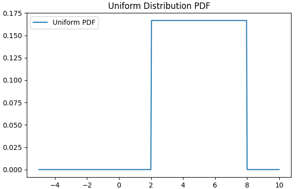
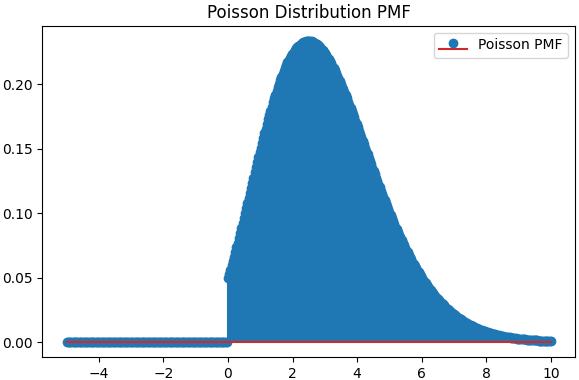
Figures (Code)
Continuous vs. Discrete	Continuous probability distributions: can take on any real value within a certain range	Discrete probability distribution	Continuous probability distributions: can take on any real value within a certain range	Discrete probability distribution: can only take on non-negative integers
Parameterization	Parameters include mean (μ) and variance (σ2).	Parameters are the minimum (a) and maximum (b) values.	The rate parameter (λ) controls the distribution's scale.	The rate parameter (λ) determines the average number of events in a fixed interval.
Shape and Symmetry	Bell-shaped and symmetric.	Rectangular and uniform, with a constant PDF within a specified range. May not be symmetric.	Right-skewed and decreasing. It models the time between events in a Poisson process. May not be symmetric.	Discrete and right-skewed. It models the number of events occurring in a fixed interval. May not be symmetric.
Support (Possible Values)	Can take any real value, from negative infinity to positive infinity.	Takes values within a specified range [a, b].	Takes positive real values (x ≥ 0).	Takes non-negative integer values (x = 0, 1, 2, ...).
Moments	Characterized by mean (μ) and variance (σ2), which determine the first and second moments.	The mean and variance are straightforward to calculate based on the parameters.	The mean and variance are determined by the rate parameter (λ).	The mean and variance are equal and determined by the rate parameter (λ).
Event/variable	Model continuous or uniform random variables.			Models counts of events.
Use Cases	Widely used for modeling data in natural and social sciences, finance, and more.	Useful for modeling scenarios with equally likely outcomes within a specified range.	Applicable to modeling the time between events in various processes (e.g., arrival times in queuing systems).	Often used to model the number of rare events occurring in a fixed interval (e.g., the number of customer arrivals at a store per hour).
Scenarios	Is more general-purpose.	Is more general-purpose.	Often used in event-based scenarios	Often used in event-based scenarios
Applications in ML	Is widely used in ML, particularly in statistical modeling and hypothesis testing. They frequently appear in applications like linear regression, clustering, dimensionality reduction, sensor measurements, financial data, and image processing.	Is less common in ML compared to other distributions. They may be used in scenarios where you want to represent equal probabilities for different outcomes, such as certain types of sampling or in simple generative models. In image processing, uniform distributions might represent pixel intensity values in certain contexts.	Is often used in ML for modeling the time between events, e.g. it can represent the distribution of inter-arrival times in queuing systems or the duration of time between failures in reliability analysis. It can also be applied to represent the time intervals between events in processes like user arrivals in a queue.	Is frequently used in ML for modeling counts of events. It's employed in applications like text analysis (e.g., modeling word counts in documents), web analytics (e.g., modeling click-through rates), and network traffic analysis. In natural language processing, Poisson distributions might be used to model the frequency of word occurrences in a document.Poisson processes are used in recommendation systems to model user actions like clicks and purchases.
Characteristics in ML	The bell-shaped curve of the Gaussian distribution is often assumed for modeling the errors in regression models (e.g., linear regression). It's also used in Gaussian Mixture Models (GMMs) for clustering.	It might be used when generating random initial values for parameters or when modeling certain types of random processes.	It may be used in survival analysis, anomaly detection, or modeling event times, such as the Poisson process and Hidden Markov Models (HMMs).	It is used in Poisson regression for count data and in various forms of recommendation systems and natural language processing tasks.
Advantages	It is well-understood and well-behaved, making it a good choice for modeling many real-world phenomena.	Is straightforward to understand and can be useful in specific situations.	It is well-suited for modeling processes where events occur at a constant rate and have a straightforward interpretation.	It's suitable for count data and scenarios where events occur at a fixed average rate over a given interval.
Disadvantages	It assume that the data is symmetric and can be unimodal, which may not always be the case in practice.	It may not accurately represent real-world data distributions, and their applications are limited compared to other distributions.	It assumes memoryless events, which may not always hold in real-world scenarios.	It assumes events are independent and stationary, which may not always be the case in practice.

Table 3867b. Applications of PDF.

============================================