=================================================================================

A Mixture of Gaussians (MoG) is a probabilistic model that represents a mixture distribution, which is a combination of multiple Gaussian (normal) distributions. In machine learning, particularly unsupervised learning, the Mixture of Gaussians model is often used for modeling complex probability distributions:

1. Gaussian Distribution (Normal Distribution): The Gaussian distribution is a continuous probability distribution defined by its mean (μ) and standard deviation (σ). It is characterized by a bell-shaped curve, and many natural phenomena follow this distribution.

2. Mixture Model: A mixture model is a probabilistic model that represents a combination (mixture) of several component distributions. Each component distribution is associated with a certain weight, representing the probability of selecting that component. The overall probability distribution is a sum of the weighted individual distributions.

3. Mixture of Gaussians (MoG): In a Mixture of Gaussians model, each component distribution is a Gaussian distribution. The overall probability distribution is a weighted sum of these Gaussian components. Mathematically, the probability density function (PDF) of a MoG is given by:

          ---------------------------- [3698a]

where:

• P(x) is the overall probability density function.
• K is the number of components (Gaussians) in the mixture.
• w_i​ is the weight associated with the i-th component, representing the probability of choosing that component.
• μ is mean.
• N(x|μ_i​, Σ_i​) is the Gaussian distribution with mean μ_i​ and covariance matrix Σ_i.

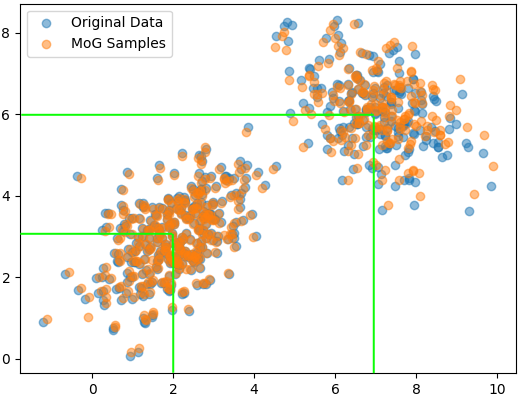
The joint probability is the product of the conditional probability of the data given the latent variable and the probability distribution of the latent variable, given by,

          ---------------------------- [3698b]

where,:

• p(x⁽ⁱ⁾|z⁽ⁱ⁾) is the conditional probability of observing x⁽ⁱ⁾ given the latent variable z⁽ⁱ⁾.
• p(z⁽ⁱ⁾) is the probability distribution of the latent variable.

    (x⁽ⁱ⁾|z⁽ⁱ⁾) ~ N (μ_i​, Σ_i) ---------------------------- [3698c]

4. Applications: Mixture of Gaussians models are commonly used for clustering and density estimation tasks in machine learning. In clustering, the model can identify underlying clusters in the data, where each cluster corresponds to one component in the mixture. In density estimation, the model can be used to estimate the probability density function of the data.
5. Parameter Estimation: The parameters of a Mixture of Gaussians model, including the means, covariances, and weights, are typically estimated using the Expectation-Maximization (EM) algorithm.

Figure 3698a shows Mixture of Gaussians (MoG) in one-dimension (1D) and two-dimension (2D). In the 1D case of the first Gaussian, the mean is 2, and for the second Gaussian (orange cluster), the mean is 7. There is no second value in the mean parameters for these one-dimensional distributions. With a two-dimensional (2D) Gaussian distribution (multivariate Gaussian), then we would specify a mean vector with two components (one for each dimension). Figure 3698a (b) shows the distinction between the blue and orange clusters which is intentionally created by using two different Gaussian distributions with distinct mean and covariance matrix parameters. The key idea behind a MoG model is that the observed data is assumed to be a mixture of multiple Gaussian distributions. Each Gaussian distribution represents a "component" of the mixture, and the overall distribution is a weighted sum of these components:

1. Gaussian Distribution 1 (Blue Cluster):

   • Mean: [2, 3]
   • Covariance Matrix: [[1, 0.5], [0.5, 1]]
   • This Gaussian distribution generates data points forming the blue cluster.
2. Gaussian Distribution 2 (Orange Cluster):
   • Mean: [7, 6]
   • Covariance Matrix: [[1, -0.5], [-0.5, 1]]
   • This Gaussian distribution generates data points forming the orange cluster.

When the Mixture of Gaussians model is fitted to the combined synthetic data, it will attempt to learn the parameters (means, covariances, and weights) of two Gaussian components, effectively capturing the structure of the original data composed of two clusters.

(a)

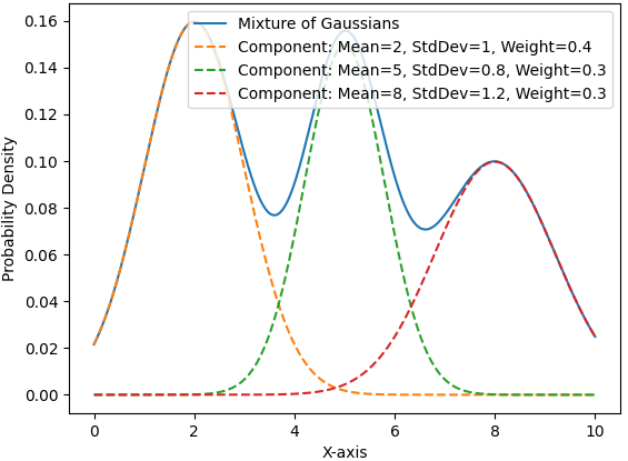
(b)

Figure 3698b shows a 1D plot of a Mixture of Gaussians, which calculates the probability density function (PDF) of the Mixture of Gaussians. The main function defines parameters for three Gaussian components, generates data points along the x-axis, and then plots both the overall Mixture of Gaussians and the individual Gaussian components.

============================================