=================================================================================
Expectation-Maximization (EM) algorithm is a general framework for finding maximum likelihood estimates of parameters in models with latent variables. The algorithm alternates between two steps: the E-step (Expectation) and the M-step (Maximization). The EM algorithm is often used in the context of Gaussian Mixture Models (GMMs), where the underlying distribution is a mixture of several Gaussian distributions.
In EM algorithm working in Gaussian Mixture Models (GMMs), for instance, for KNN (K-Nearest Neighbours), EM provides a probabilistic or "soft" assignment of data points to different clusters or components, and it incorporates probabilities rather than making a hard assignment based on the closest cluster center. Additionally, the update equations for the cluster parameters involve weighted averages based on these probabilities.
In a GMM, each data point is considered to be generated by one of several Gaussian distributions, and the EM algorithm iteratively estimates the parameters of these Gaussian distributions. The probability that a data point x(i) belongs to the j-th Gaussian component is given by wj(i) as discussed in Mixture of Gaussians (MoG). Then, the main steps of EM algorithm working in GMMs are:
i) Soft Assignment:
Instead of assigning a data point exclusively to the cluster with the maximum probability, EM assigns it to all clusters with some probability. The "softness" of the assignment is captured by these probabilities. Mathematically, the assignment is based on the responsibility wj(i):
 --------------------------------- [3695a] --------------------------------- [3695a]
ii) Parameter updates:
The cluster parameters, such as the mixing coefficients (ϕj), means (μj), and covariances (εj), are updated using weighted averages. The weights are the responsibilities wj(i), indicating the likelihood of a data point belonging to a specific cluster:
ii.a) Mixing coefficient update:
 ----------------------------------------------------------------- [3695b] ----------------------------------------------------------------- [3695b]
ii.b) Mean update:
 ---------------------------------------------- [3695c] ---------------------------------------------- [3695c]
ii.c) Covariance update (for a full covariance matrix):
 ---------------------------------------------- [3695d] ---------------------------------------------- [3695d]
where,
- p(x(i), z(i); ϕ, μ, ε) is the joint probability of observing x(i) and its corresponding latent variable z(i) given the parameters ϕ, μ, and ε.
- ϕj represents the probability that a randomly selected data point belongs to the j-th component of the mixture. It is estimated by counting the proportion of data points assigned to the j-th component.
- μj represents the mean of the distribution associated with the j-th component of the mixture. It is estimated by computing the weighted average of the observations assigned to the j-th component, where the weights are the probabilities of belonging to that component.
These equations illustrate that the updates are influenced by the probabilities wj(i), which reflect the degree of association of each data point with each cluster. The soft assignment and weighted updates are key features that distinguish EM-based clustering, like GMMs, from "hard" clustering methods.
The basic steps of deriving the EM algorithm using Multivariate Gaussian properties, specifically in Gaussian Mixture Models are:
-
Define the Model:
- Assume that the observed data is generated from a mixture of multiple multivariate Gaussian distributions.
- Define the parameters of the model, including the mean vectors, covariance matrices, and mixing coefficients for each Gaussian component.
- Derive P(x,z). The goal is to derive the joint distribution of the observed data (x) and the latent variables (z). The joint distribution is a key component in the derivation of the EM algorithm.
 ------------------------------- [3695de] ------------------------------- [3695de]
 ----------------------------------------- [3695df] ----------------------------------------- [3695df]
 ------------------------------------------------------- [3695dg] ------------------------------------------------------- [3695dg]
 ------------------------------------------------------- [3695dh] ------------------------------------------------------- [3695dh]
The "0" in the partition matrix μx,z in Equation 3695dh is d-dimensional, and μ n-dimensional.
Equation 3695df indicates that the joint normal distribution of the latent variable z and the observed variable x follows a multivariate Gaussian distribution with a mean vector μx,z and a covariance matrix ε.
Expected x is given by factor analysis, which is,
 ------------------------------------------------ [3695di] ------------------------------------------------ [3695di]
We also have,
 ------------------------------------------------ [3695dj] ------------------------------------------------ [3695dj]
 -------------------------- [3695dk] -------------------------- [3695dk]
where,
 is a block, which represents the covariance matrix of the latent variable z. The covariance matrix is computed as the expectation of the outer product of z - Ez . is a block, which represents the covariance matrix of the latent variable z. The covariance matrix is computed as the expectation of the outer product of z - Ez .
 and and  are blocks, which are cross-covariance matrices between the latent variable z and the observed variable x. are blocks, which are cross-covariance matrices between the latent variable z and the observed variable x.
 is a block, which represents the covariance matrix of the observed variable x. is a block, which represents the covariance matrix of the observed variable x.
Ez and Ex typically denotes the expectations with respect to the distributions of z and x, respectively.
The first column in Equations 3695dj and 3695dk is d-dimensional, while the second column is n-dimensional. Those two equations represent a block matrix representation for the covariance matrix ε in a multivariate distribution. This representation is derived based on the law of total covariance or the law of iterated covariance.
In the EM algorithm, particularly when dealing with Gaussian Mixture Models (GMMs), the covariance matrix ε is often expressed as a block matrix. This representation helps in expressing the covariance structure of the joint distribution of the latent and observed variables.
Furthermore, we have,
 ------------------------------------------------ [3695dl] ------------------------------------------------ [3695dl]
 ------------------------------------------------ [3695dm] ------------------------------------------------ [3695dm]
If E(z) = 0 and E(ε) = 0, then Ex = μ, so that we have,
 --------------------- [3695dn] --------------------- [3695dn]
 --------------------------- [3695do] --------------------------- [3695do]
 --------------------------- [3695dp] --------------------------- [3695dp]
where,
-- The first term in Equation 3695dp represents the covariance matrix between Λz and itself. If z is a random variable with zero mean, then we have,
 ------------------------ [3695dq] ------------------------ [3695dq]
Var(z) refers to the variance of the random variable z. The variance is a measure of the spread or dispersion of a random variable, and it is defined as the expected value of the squared deviation from the mean.
If z follows a normal distribution, then the variance is simply the square of the standard deviation. In the case of z ~ N(0, 1) (a standard normal distribution), then we have,
 ------------------------ [3695dqd] ------------------------ [3695dqd]
If z follows a different distribution with mean μz and variance σz2 , then we have,
 ------------------------ [3695dqe] ------------------------ [3695dqe]
Moreover, f z is a univariate normal distribution (z ~ N(0, 1)), then Var(z) = 1 (a scalar). However, if z is a multivariate normal distribution (z ~ N(μ, Σ)), where μ is the mean vector and Σ is the covariance matrix, then Var(z) is the covariance matrix Σ.
 ------------------------ [3695dqf] ------------------------ [3695dqf]
If Σ is the identity matrix, then Var(z) would indeed be the identity matrix.
-- The second term in Equation 3695dp represents the cross-covariance between Λz and ε. If ε is assumed to be uncorrelated with Λz and has zero mean, then we have,
 .-------------------- [3695ds] .-------------------- [3695ds]
-- This third term in Equation 3695dp represents the cross-covariance between ε and z. If z and ε are assumed to be uncorrelated, then we have,
 ------------------ [3695dt] ------------------ [3695dt]
-- This fourth term in Equation 3695dp represents the covariance matrix of ε. It is not zero in general, but it is equal to φ.
With similar equation analysis for other terms in Equation 3695dj, then Equation 3695dj becomes,
 ------------------ [3695du] ------------------ [3695du]
This obtained equation can be inserted into Equation 3695df. Now, the goal is to maximize the log-likelihood of the observed data. The log-likelihood involves parameters like μx,z, Λ (which presumably relates to the covariance structure), and ε (which may involve the covariance matrix Ψ). Then, the next strategy involves taking derivatives of the log-likelihood with respect to the parameters. Setting the derivatives to zero is a common approach to finding the maximum likelihood estimates (MLE) because it identifies points where the slope of the log-likelihood is zero. The observation that there is no closed-form solution implies that the system of equations formed by setting the derivatives to zero doesn't yield a simple algebraic solution. This is a common challenge in many statistical models, especially those involving latent variables and complex parameter dependencies. In cases where closed-form solutions are not feasible, optimization techniques, such as iterative algorithms like the EM algorithm or gradient-based optimization methods, are often employed to numerically find the parameter values that maximize the log-likelihood. However, the absence of a closed-form solution doesn't necessarily hinder the applicability of the model or the optimization process, but it may require numerical methods to find the optimal parameter values.
- E-step (Expectation):
- Compute the posterior probabilities (responsibilities) of each data point belonging to each Gaussian component. In this step, the goal is to compute the expected value of the latent variables given the observed data and the current parameter estimates. This involves calculating the conditional probabilities of the latent variables given the observed data and the current parameter values. This is done using Bayes' theorem. The conditional probability is given by,
 ----------------------------------- [3695dv] ----------------------------------- [3695dv]
The expression Qi(z(i)) is often referred to as the "responsibility" of the i-th data point for the different components in a mixture model.
The conditional normal (Gaussian) distribution is given by,
 -------------------------- [3695dw] -------------------------- [3695dw]
where,
z(i)|x(i) denotes the random variable z(i) given the observed data x(i). It represents the conditional distribution of the latent variable z(i) given the specific observed data point x(i).
The "~" symbol means "is distributed as" or "follows the distribution."
 specifies the type of distribution, which is a multivariate normal distribution. The parameters of this distribution are: specifies the type of distribution, which is a multivariate normal distribution. The parameters of this distribution are:
 is the mean vector of the conditional distribution. It represents the expected value of z(i) given x(i). is the mean vector of the conditional distribution. It represents the expected value of z(i) given x(i). is the covariance matrix of the conditional distribution. It characterizes the spread and correlation of z(i) given x(i). is the covariance matrix of the conditional distribution. It characterizes the spread and correlation of z(i) given x(i).
As discussed in page3864, for a conditional distribution of x3 given x2 in a multivariate gaussian distribution, we have,
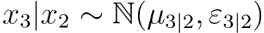 ------------------------------------------- [3695dxc] ------------------------------------------- [3695dxc]
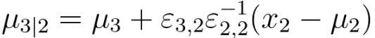 ----------------------- [3695dxd] ----------------------- [3695dxd]
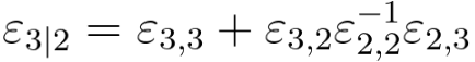 -------------------------------- [3695dxe] -------------------------------- [3695dxe]
Based on Equation 3695dxd, the mean vector of the conditional distribution z(i)|x(i) under certain assumptions is given by,
 -------------------------- [3695dxf] -------------------------- [3695dxf]
where,
- 0 is a vector of zeros.
- Λ is a matrix associated with the linear transformation from the latent variable z to the observed variable x.
- μ is the mean vector of the joint distribution of z and x.
- I is the identity matrix.
On the other hand, based on Equation 3695dxe, the formula for the covariance matrix of the conditional distribution z(i)|x(i) under certain assumptions can be given by,
 -------------------------- [3695dxg] -------------------------- [3695dxg]
where,
- I is the identity matrix.
- Λ is a matrix associated with the linear transformation from the latent variable z to the observed variable x.
- Ψ is a covariance matrix associated with the noise or error term in the relationship between z and x.
Therefore, in E-step, to compute Qi, we need to compute Equations 3695dxf and 3695dxg first.
In this step, we will need to compute,
 -------------------------- [3695dxh] -------------------------- [3695dxh]
We know Qi is Gaussian distribution, so that we can use expected value formula,
 -------------------------- [3695dxi] -------------------------- [3695dxi]
Equation 3695dxi represents the expectation of the latent variable z with respect to its marginal distribution p(z). This is the unconditioned expectation of z. In the current case, Qi(z(i)) is a Gaussian distribution, then the integral in Expression 3695dxh can be computed using the mean, in Equation 3695dxf, and covariance matrix, in Equation 3695dxg, of the Gaussian distribution.
Therefore, with the discussion above, if Qi(z(i)) is a Gaussian distribution with mean and covariance matrix , then the expectation is equal to the mean , namely,
 -------------------------- [3695dxj] -------------------------- [3695dxj]
It should be highlighted that the condition for Equation 3695dxj to be correct is that Qi(z(i)) is a Gaussian distribution. Specifically, Qi(z(i)) should be a multivariate Gaussian distribution with a valid mean vector and covariance matrix. This equation is advantageous in EM algorithm, particularly in the E-step:
i) Simplification of Expectation Calculations:
- When the conditional distribution Qi(z(i)) is Gaussian, this equation simplifies the calculation of the expectation. Instead of integrating over the entire distribution, which is the exponential probability density function (see page3864), the mean of the Gaussian distribution provides a straightforward and computationally efficient way to represent the expectation.
ii) Closed-Form Expression:
- Gaussian distributions have convenient properties that lead to closed-form expressions for their expectations. The mean of a Gaussian distribution is a summary statistic that fully captures the first moment of the distribution.
iii) Compatibility with EM Algorithm:
- The EM algorithm involves iteratively updating estimates of latent variables and parameters. The simplification provided by the equation aligns well with the iterative nature of the algorithm, making it computationally efficient and numerically stable.
iv) Connection to Maximum Likelihood Estimation (MLE):
- In the E-step of EM, the goal is to compute expected values that are later used in the M-step to maximize the likelihood function. The use of the mean of a Gaussian distribution simplifies the expressions involved in the MLE process.
v) Interpretability:
- The mean of a Gaussian distribution has a clear interpretation as the center or expected value of the distribution. This can enhance the interpretability of the conditional expectations in the context of the model.
However, the application of the existing integral (Equation 3695dxj) requires certain conditions to be met, and understanding these conditions is essential for the correctness of the algorithm:
i) Gaussian Assumption:
- The equation assumes that the conditional distribution Qi(z(i)) is Gaussian. If this assumption does not hold, attempting to use this simplification may lead to incorrect results.
ii) Completeness of Moments:
- The simplification relies on the completeness of the first moment (mean) of the distribution. This may not hold for all types of distributions.
iii) Analytical Form:
- The integral simplification is more likely to be applicable when the conditional distribution has a known and manageable analytical form. If the form is complex or unknown, numerical methods may be necessary.
iv) Validity of Covariance Matrix:
- The equation assumes the validity of the covariance matrix in the Gaussian distribution. If the covariance matrix is singular or ill-conditioned, the inversion involved in the equation may be problematic.
v) Context of the Model:
- The applicability of the existing integral depends on the specific probabilistic model being used. Understanding the assumptions and limitations of the model is essential.
vi) Numeric Stability:
- When working with numerical computations, particularly in machine learning, one should be mindful of numerical stability issues. This includes handling situations where inversion of matrices might be numerically challenging.
- The responsibility of the ith data point for the j-th Gaussian component is given by:
 ----------------------------------- [3695e] ----------------------------------- [3695e]
where πj is the mixing coefficient, μj is the mean vector, Σj is the covariance matrix of the jth Gaussian component, and K is the total number of components.
- M-step (Maximization):
- Update the parameters of the model based on the computed responsibilities.
- The parameter update can be given by,
 ---------------------- [3695fh] ---------------------- [3695fh]
 ---------------------- [3695fi] ---------------------- [3695fi]
The reasons of having this equation are:
i) Objective Function:
- The goal of the M-step in the EM algorithm is to maximize the expected log-likelihood, which is expressed as the sum over all data points i of the expected log-likelihood for each data point.
ii) Expectation:
- The expectation is taken with respect to the conditional distribution Qi(z(i)), which represents the posterior distribution of the latent variable given the observed data.
 represents the expectation with respect to the conditional distribution Qi(z(i)). This expectation is taken over the latent variable z(i) according to the distribution Qi. represents the expectation with respect to the conditional distribution Qi(z(i)). This expectation is taken over the latent variable z(i) according to the distribution Qi.
iii) Log-Likelihood Ratio:
- The expression inside the logarithm is the ratio of the joint distribution P(x(i), z(i)) to the conditional distribution Qi(z(i)). This ratio is a measure of how well the current model (with parameters θ) explains the observed data.
iv) Integration over Latent Variables:
- The integral in Equation 3695fh involves integrating over the latent variable z(i) according to the conditional distribution Qi(z(i)). This step accounts for uncertainty in the latent variable.
v) Summation over Data Points:
- The sum ∑i ensures that the optimization objective includes contributions from all data points, making the objective a sum of expected log-likelihoods across the entire dataset.
- Update the mean vectors, covariance matrices, and mixing coefficients using the weighted sum of the data points, where the weights are the responsibilities:
 ----------------------------------- [3695f] ----------------------------------- [3695f]
 ----------------------------------- [3695g] ----------------------------------- [3695g]
 ----------------------------------- [3695h] ----------------------------------- [3695h]
- Repeat:
- Repeat the E-step and M-step until convergence. Convergence can be determined by monitoring changes in the log-likelihood or other convergence criteria.
============================================
|
