=================================================================================

In machine learning, the choice of the loss function, which measures the error or the difference between predicted and actual values, depends on the specific problem and the characteristics of the data.

Squared error (also known as Mean Squared Error or MSE) is a commonly used loss function for several reasons:

1. Simplicity: Squared error is a simple and differentiable function. This makes it easy to work with mathematically, and it allows for efficient optimization techniques like gradient descent to find the model parameters that minimize the error.

2. Convexity: The squared error loss function is convex, which means it has a single global minimum. This property makes it easier to find the optimal model parameters, as optimization algorithms are guaranteed to converge to the global minimum.

3. Emphasis on Outliers: Squared error places more emphasis on large errors or outliers compared to other loss functions like absolute error. In some cases, you may want the model to penalize large errors more severely, especially if outliers are significant or have a particular meaning in your application.

4. Statistical Assumptions: Squared error loss is closely related to the maximum likelihood estimation (MLE) under the assumption of normally distributed errors. Many statistical models assume normally distributed errors, making squared error a natural choice.

Using the fourth power (quartic) of errors as a loss function in machine learning is relatively uncommon compared to Mean Squared Error (MSE) or absolute error (L1 loss), and it has specific characteristics and use cases:

1. Sensitivity to Outliers: Using the fourth power of errors places even more emphasis on outliers than MSE does. Large errors are penalized much more severely than with MSE, which means that the model will be extremely sensitive to extreme outliers. If your dataset contains significant outliers that you want to heavily penalize, this may be a reason to consider using a fourth-power loss.

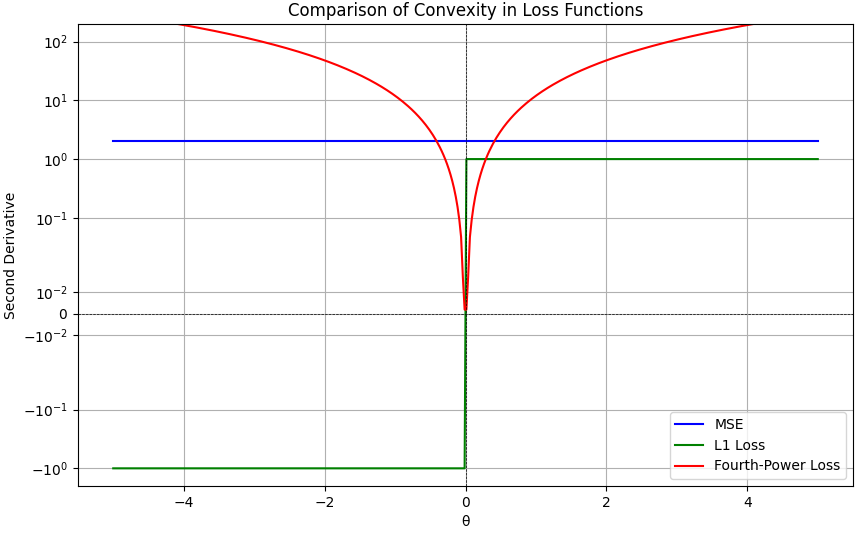
2. Mathematical Properties: The fourth-power loss function is a non-convex function (see page3914), meaning it may have multiple local minima, making it more challenging to optimize. This can lead to optimization problems when training models, and it may require more sophisticated optimization techniques.

3. Interpretability: Using the fourth power of errors can make the loss function less interpretable compared to MSE or absolute error. In machine learning, interpretability is often an important consideration, especially in applications where model decisions need to be understood and justified.

4. Domain-Specific Considerations: In some specific domains or applications, using a fourth-power loss function may have a theoretical or practical basis. For instance, in certain physical or engineering problems, the error may have a physical significance that aligns with a fourth-power loss function.

Using the absolute value (L1 loss) as a loss function in machine learning has its own set of advantages and use cases compared to Mean Squared Error (MSE) or the fourth power of errors. Here are some reasons why you might choose absolute value loss:

1. Robustness to Outliers: The L1 loss is less sensitive to outliers than MSE. In MSE, large errors are squared and penalized more heavily, which can make the model overly sensitive to extreme values in the dataset. In contrast, the L1 loss treats all errors linearly, so it is more robust in the presence of outliers. If your dataset contains significant outliers and you want the model to be less affected by them, L1 loss can be a good choice.

2. Sparsity: L1 loss encourages sparsity in the model's predictions. When using L1 regularization (Lasso), it tends to push some model coefficients to exactly zero, effectively selecting a subset of the most important features. This property can be beneficial for feature selection or when you want a simpler and more interpretable model.

3. Median Estimation: L1 loss is closely related to the median. Minimizing the L1 loss is equivalent to finding the median of the target variable, which can be valuable in situations where you want to predict a median-like value rather than the mean (as in the case of MSE).

4. Robust Regression: L1 loss is often used in robust regression techniques, such as robust linear regression and quantile regression, where the goal is to model the central tendency of the data in a more robust way that is less affected by outliers.

5. Non-Gaussian Errors: In cases where the assumptions of normally distributed errors underlying MSE are not valid, L1 loss can be a more appropriate choice, as it does not rely on Gaussian assumptions.

Assuming the equation below:

          --------------------------------- [3880a]

where,

         ε⁽ⁱ⁾ is the un-modeled effects or random noise.

A few common models for ε(i) depending on the specific cases are:

1. Gaussian (Normal) Distribution: Assuming that the errors follow a Gaussian distribution (also known as normal distribution) is a common choice. In this case, you can assume that,

            ε(i) ~ N(0, σ²) ------------------------------------------------------------------------------- [3880b]

                      where,          

             σ² represents the variance of the errors.

            
2. Homoscedasticity: This assumption implies that the variance of ε(i) is constant across all observations. In other words, σ² does not depend on the values of y⁽ⁱ⁾. If the assumption of homoscedasticity is violated, you might consider using a heteroscedasticity model where the variance of ε(i) varies with y⁽ⁱ⁾.
3. Autocorrelation: In time series analysis, you might consider models that account for autocorrelation in the errors, especially if the observations are not independent over time. Examples include autoregressive integrated moving average (ARIMA) models or autoregressive conditional heteroscedasticity (ARCH) models.
4. Non-Gaussian Distributions: Depending on the nature of your data, you might consider models that assume non-Gaussian distributions for ε(i). For example, if your data is count data, you might use a Poisson or negative binomial distribution.
5. Mixed-Effects Models: When dealing with hierarchical or nested data, you might use mixed-effects models that account for both fixed effects (systematic variations) and random effects (random variations) in the data. The random effects can capture un-modeled variation between groups or clusters.
6. Machine Learning Models: In machine learning, you can use various models, such as decision trees, random forests, support vector machines, or neural networks, to capture complex relationships between features and the error term ε(i).

If the error term ε(i) is assumed to follow a Gaussian (Normal) distribution, then the probability density function (PDF) of ε(i) is given by the normal distribution formula:

          --------------------------------- [3880c]

Where:

• f(ϵ(i)) is the probability density function of ε(i).
• μ is the mean (expected value) of ε(i).
• σ² is the variance of ε(i).
• ​ is a normalization constant.

In this formula, μ represents the center or location of the distribution, and σ²represents the spread or dispersion of the distribution. The PDF describes the likelihood of observing a particular value of ε(i) in the context of a normal distribution. If ε(i) is normally distributed, it means that most of the observations are likely to be close to the mean (μ), and the distribution is symmetric and bell-shaped. The spread of the distribution is determined by the variance (σ²). Larger values of σ²result in a wider distribution, while smaller values result in a narrower distribution.

Assuming variables are independent and identically distributed, then,

          --------------------- [3880d]

where,

          θ^Tx⁽ⁱ⁾ the mean (expected value) of y⁽ⁱ⁾ as it can be known from Equation 3880c.

Note that the semicolon ";" in Equation 3880d can be changed to ","; otherwise it will conditioning θ, which is incorrect. ";" means that it is parameterized by θ (refer to page3960):

Similar to Equation 3880b, we have,

          ---------------------------- [3880e]

Here, the left hand side is random variables and the right hand side represents the distribution.

Figure 3880a shows the comparison between mean squared error (MSE), absolute error (L1 Loss) and fourth-power loss, and Figure 3880b shows convexity of loss functions.

(a)

(b)

(c)

Figure 3880b Convexity of loss functions (Python code).

============================================