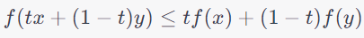
=================================================================================

The convexity of loss functions is an important concept in optimization and machine learning. Convex loss functions have desirable properties because they ensure that optimization algorithms converge to global minima. A function is considered convex if, for any two points x and y in its domain and any value of t between 0 and 1, the following inequality holds:if:

          ------------------------------ [3914a]

For the fourth-power loss function L(x) = x⁴, you can easily see that it is not convex::

1. Consider x = −1 and y = 1. Both x and y are in the domain of L(x), and the line segment connecting them is the horizontal line segment from (−1,1) to (1,1).

2. Let's evaluate L(x) at these points:
   • L(−1) = (−1)⁴ = 1
   • L(1) = (1)⁴ = 1
3. Then, let's evaluate L(tx + (1 − t)y) for t = 0.5 (the midpoint of the line segment), which is the left side of the convexity inequality:
   • L(0.5(-1) + 0.5(1)) = L(0) = (0)⁴ = 0
4. Then, let's evaluate the right side of the convexity inequality:
   • 0.5L(-1) + 0.5L(1) = 0.5 + 0.5 = 1.

The comparison of the convexities of the three loss functions is listed below:

1. Fourth-Power Loss Function (Red Curve):

   • The fourth-power loss function is defined as L(θ) = θ⁴, where θ is a scalar parameter.
   • The second derivative of this loss function is given by: L''(θ) = 12θ².
   • As shown in the plot in Figure 3914, the second derivative of the fourth-power loss function is always positive for all values of θ, except at θ = 0 where it is equal to zero.
   • Since the second derivative is positive everywhere except at a single point (θ = 0). Convexity requires that the second derivative is non-negative for all θ in the function's domain. At θ = 0, the second derivative is zero, which means it does not satisfy the condition of being strictly positive for all θ ≠0. As a result, by the standard mathematical definition of convexity, the fourth-power loss function L(θ) = θ⁴ is not considered convex. It is a non-convex function because it fails to satisfy the convexity inequality for all θ in its domain.
2. Squared Error (MSE) Loss Function (Blue Curve):
   • The squared error loss function is defined as L(θ) = θ², where θ is a scalar parameter.
   • The second derivative of this loss function is given by: L''(θ) = 2.
   • The second derivative is a constant (2) and is always positive.
   • Therefore, the squared error loss function is convex. Its second derivative being a constant is indicative of a convex function.
3. L1 Loss Function (Green Curve):
   • The L1 loss function is defined as L(θ) = |θ|, where θ is a scalar parameter.
   • The second derivative of this loss function is given by: L''(θ) = 0 everywhere except at θ = 0, where the second derivative is undefined.
   • The second derivative is zero almost everywhere except at θ = 0.
   • The L1 loss function is not globally convex because it is not differentiable at θ = 0. The absence of a defined second derivative at θ = 0 makes it a non-convex function.

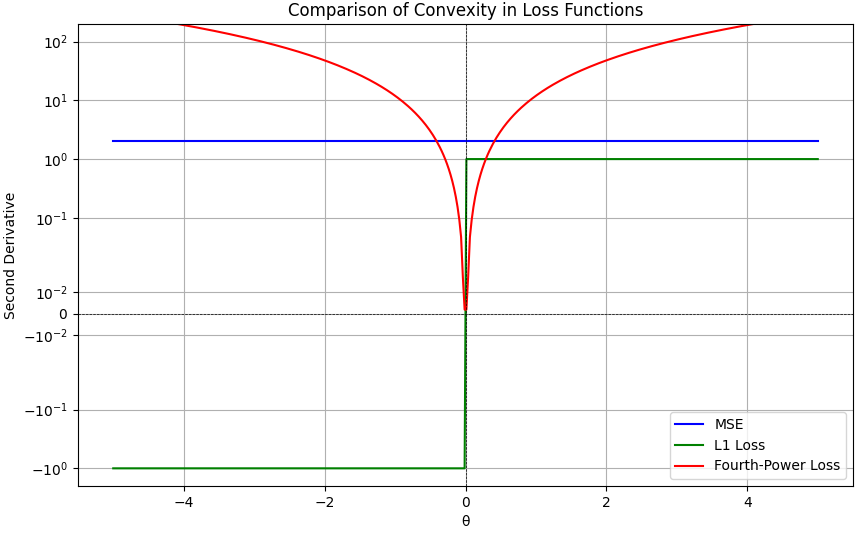
Figure 3914. Convexity of loss functions (Python code).

Convex optimization is a mathematical field that deals with the problem of finding the best solution to a convex optimization problem. Convex optimization problems have certain characteristics that make them solvable efficiently and reliably. Here are the key components and concepts related to convex optimization algorithms:

1. Convex Functions: Central to convex optimization are convex functions. A function is considered convex if, for any two points in its domain, the line segment connecting these points lies above the graph of the function. In other words, a function f(x) is convex if and only if:

   ------------------------------ [3914b]

   where x_1 and x_2 are points in the domain of f, and 0 <= t <= 1.

2. Convex Sets: In addition to convex functions, convex optimization deals with convex sets, which are sets that contain all the line segments connecting any two points within the set. Convex optimization problems typically involve finding a point within a convex set that optimizes a convex function.

3. Convex Optimization Problems: Convex optimization problems can be stated as follows:

   • Minimization Problem: Minimize a convex function f(x) subject to certain linear equality and inequality constraints:

   ------------------------------ [3914c]

Here, x is the optimization variable, f(x) is the objective function to be minimized, Ax = b represents equality constraints, and Gx ≤ h represents inequality constraints.

4. Convexity Ensures Global Optimality: One of the key advantages of convex optimization is that it guarantees that any local minimum of a convex function is also a global minimum. This property makes convex optimization problems easier to solve because you can be confident that the solution you find is indeed the best possible.
5. Convex Optimization Algorithms: Several algorithms are used to solve convex optimization problems, including but not limited to:
   • Linear Programming (LP): Used for linear objective functions and constraints.
   • Quadratic Programming (QP): Deals with quadratic objective functions and linear constraints.
   • Semidefinite Programming (SDP): Extends convex optimization to semidefinite constraints.
   • Interior-Point Methods: These are iterative methods that solve convex optimization problems by moving toward the interior of the feasible region.
   • Gradient Descent: Used for smooth convex functions, where the gradient points in the direction of steepest descent.
6. Applications: Convex optimization has a wide range of applications in various fields, including machine learning (support vector machines, logistic regression, etc.), finance (portfolio optimization), engineering (control systems, signal processing), and operations research (resource allocation, network flow optimization), among others.

Convex optimization algorithms are mathematical techniques used to find the optimal solution to convex optimization problems, where the objective function is convex, and the constraints define a convex feasible region. The convexity property ensures that these algorithms can efficiently find globally optimal solutions, making them valuable in a variety of practical applications.

============================================

Both convex functions and a shaded convex set. Code:
         
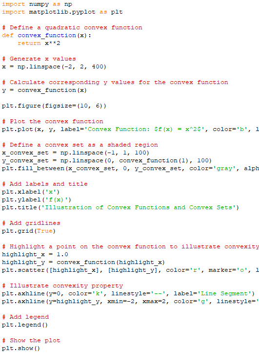
       Output:    
         

============================================