 |
||||||||||||||||||||||||||||||||||
Negative Binomial Yield Model (with Random-but-Clustered Defects/Fails) - Integrated Circuits and Materials - - An Online Book - |
||||||||||||||||||||||||||||||||||
| Integrated Circuits and Materials http://www.globalsino.com/ICsAndMaterials/ | ||||||||||||||||||||||||||||||||||
| Chapter/Index: Introduction | A | B | C | D | E | F | G | H | I | J | K | L | M | N | O | P | Q | R | S | T | U | V | W | X | Y | Z | Appendix | ||||||||||||||||||||||||||||||||||
================================================================================= If the distribution of the defects/fails is random, but clustered, then the negative binomial yield model can be used. In this case, it can be assumed that the likelihood of an
event occurring at a given location increases linearly with the number of events
that have already occurred at that location. [1] In this model, the probability that one die contains k defects follows negative
binomial distribution, [2] It can be known that: As an example, assuming a single IC chip has an average of 0.001 faults per die, if the negative binomial yield model of Equation 4304b is applied, and the yield of a die with 500 of these ICs is
equal to, Table 4304 shows estimated yield for 0 = 0.5, 1.0, 2.0, ∞ with different yield models.
============================================
[1] Ferris-Prabhu, A.V., "Models for Defects and Yield," in Defect and Fault Tolerance in VLSI Systems, edited by Koren, I., 1989, pp 33-46. [2] Way Kuo, Wei-Ting Kary Chien and Taeho Kim, Reliability, Yield, and Stress Burn-In: A Unified Approach for Microelectronics Systems Manufacturing & Software Development, 1998. [3] Stapper, C.H., "Fact and fiction in yield modeling," Microelectronics Journal, 20, (1/2), 1989, pp 129-151. [4] Stapper, C.H., "Defect density distribution for LSI yield calculations," IEEE 7ransactions on Electron Devices, ED-20, Jul. 1973, pp 655-657.
|
||||||||||||||||||||||||||||||||||
| ================================================================================= | ||||||||||||||||||||||||||||||||||
|
|
||||||||||||||||||||||||||||||||||
 -------------------------------------- [4304a]
 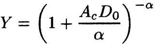 -------------------------------------------------------------------------------------------------------- [4304b]