Radial Distribution Function (RDF) from Electron Diffraction Patterns - Practical Electron Microscopy and Database - - An Online Book - |
|||||||||||||
| Microanalysis | EM Book http://www.globalsino.com/EM/ | |||||||||||||
| ================================================================================= | |||||||||||||
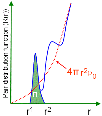
Similar to pair distribution function (PDF), radial distribution function (RDF, R(r)) is also related to the Fourier transform of the measured scattering intensity S(Q). The pair distribution function, including the full information about the three-dimensional (3-D) structure, is difficult to plot because of the dependence on vectors. Therefore, in practice, this information is reduced to the radial distribution function. R(r)dr provides the number of atoms in the annulus of thickness dr at distance r from the origin atom. RDF from electron diffraction patterns has been used to provide the interatomic distances and their distributions of amorphous and nanocrystalline materials. The profiling of the one-dimensional (1-D) RDF with electron diffraction is similar to X-ray diffraction RDF that presents the distance correlation between a pair of atoms. The concept of RDF is very important, for instance, when we study the thermodynamics of vibrational, magnetic, electronic and superconducting excitations in amorphous metals. The radial distribution function can be given by, The number of atoms in a spherical shell between r and r + dr from the origin atom is given by, The RDF tends to become a smooth parabola at large values of r as shown in Figure 1426a (a).
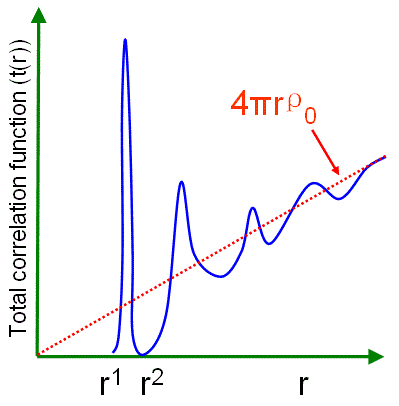
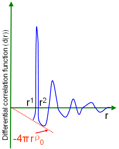
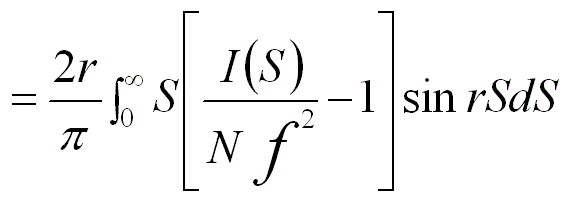
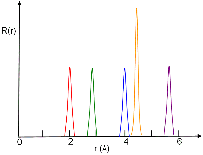
The number of neighbors to the origin atom residing between r1 and r2 can be given by the area (e.g. the green area in Figure 1426a (a)) under the peak, In some cases, RDF is plotted as 4πr2[ρ(r) - ρ0] versus r when the parabola has been subtracted out. Based on Warren theory [1], we can have, where, Furthermore, reduced RDF is the third method of plotting the data. The reduced RDF is also called total correction function t(r) (see Figure 1426a (b)), given by, Similarly, differential correlation function d(r) (see Figure 1426a (c)) is given by, The peaks in the data plots in Figures 1426 (b) and (c) can be defined more precisely and thus the integration of the areas is much easier than in Figures 1426 (a) for determining the coordination number. In the case with Equations 1426d to 1426f, the RDF oscillates about the abscissa. In practice, RDF (as well as Partial Radial Distribution Function, PRDF) can most efficiently be determined by computer-modeling the amorphous systems, only by counting the numbers of atoms of kind B that are at a distance between r and r+dr from an origin atom of kind A, and then averaging over all atoms A. In diffraction experiments (X-ray, neutron or electron diffraction, or their combinations), S in Equation 1426g is the scattered intensity. After normalization, we can obtain the coherent intensity Icoh(S) as a function of S. The Fourier transform of the total structure factor F(S) is then simply the differential correlation function d(r) in Equation 1426i. Figure 1426b shows the schematic illustrations of generation of pair distribution function from a two-dimensional (2-D) crystal and the corresponding peaks in the radial distribution function.
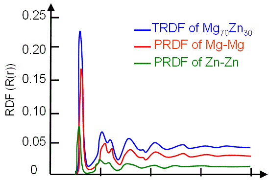
As an examlpe, Figure 1426c shows the computer-simulated total radial distribution function (TRDF) for the amorphous Mg70Zn30 and partial radial distribution functions (PRDFs) corresponding to the Mg-Mg and Zn-Zn correlations, respectively.
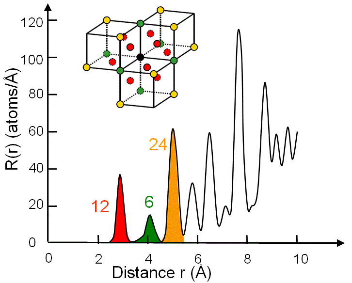
Figure 1426d shows the radial distribution function R(r), of the fcc gold (Au) crystal, from the black (origin) atom at room temperature. The RDF peaks with the atoms in the different colors correspond to the atoms in the same color in the atomic structure of the inset.
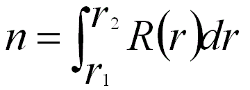
Figure 1426d. Radial distribution function R(r) of fcc gold (Au) at room temperature. In both ordered (e.g. crystal) and disordered (e.g. amorphous) states, R(r) can be used to evaluate the average number (n) of atoms located between r1 and r2, Note that for a system with multiple types of elements, it is usual to find atoms of a different type B around the origin atom A. In general, the RDF analysis is important for the study of non-crystalline solids. It describes the mutual relationship between the location of various atoms, and thus can be used to provide the degree of long-range atomic ordering in amorphous materials, the distribution of interatomic distances, and the average nearest-neighbor coordination number of amorphous materials, polycrystalline materials, liquids, and gases. RDFs can be experimentally measured after Fourier transformation of neutron or electron diffraction or X-ray diffraction (XRD) data. The calculation of RDF is a well-known method for quantitative analysis of diffuse diffraction diagrams of amorphous samples. [3-4] For instance, the position of the first maximum of RDF represents the most probable distance between neighbouring atoms and decreases from 2.75 to 2.62 Å in films with an increasing Si-content from 60 to 75 at%. [5]
[1] B.E. Warren, The Diffraction of X-Rays in Glass. Physical Review 45: 657, (1934).
|
|||||||||||||
| ================================================================================= | |||||||||||||
|
|
|||||||||||||
 ----------------------[1426f]
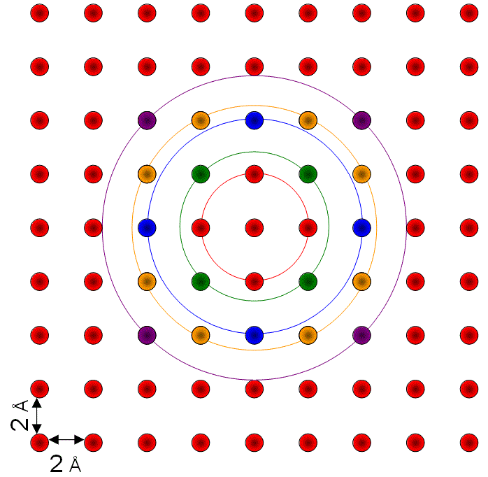
 ---------------------- [1426j]