=================================================================================
Ronchigram can be described as a shadow image, or microdiffraction pattern of a specimen that is projected onto an infinitely distant plane by means of an electron beam focused on or near the specimen as shown in Figure 3590a. Each point of the disc in Ronchigram corresponds to a tilted ray in the probe. At focus, the probed area is the smallest and the image blows-up to "infinity" magnification. The image reverses from underfocus to overfocus.
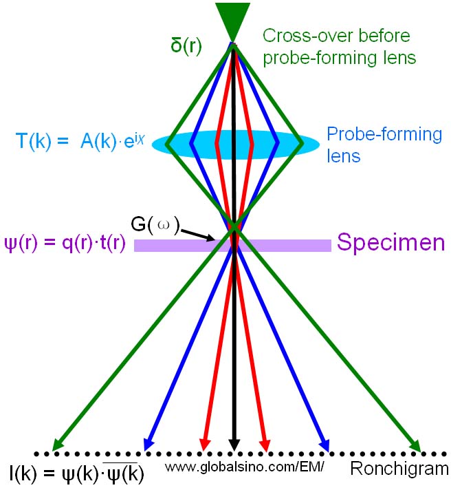
Figure 3590a. Schematic illustration of Ronchigram formation.
Near the focal point, the formed image is heavily distorted by the aberrations of the probe-forming lens. Therefore, the Ronchigram is also the convergent beam diffraction pattern of an amorphous region or a crystal where the aperture is much larger than the Bragg angles. Note that depending on the context and who is talking about it, Ronchigram can also be called the Gabor hologram or the central zero-order disc of the convergent beam electron diffraction pattern.
The Ronchigram contains not only abundant information on the specimen but also on the STEM operating conditions and its probe-forming optics [1]. Because the intensity of Ronchigram, formed at the Fraunhofer diffraction plane, varies significantly with angle, and this variation is a very sensitive function of lens aberrations and defocus [1], Ronchigram is a very useful way to characterize and optimize the electron probe in STEM mode.
Cowley and others had theoretically studied the formation of Ronchigram patterns. [1, 2, 6-9] We can consider that a probe-forming lens has a transfer function T(k),
T(k) = A(k) eiχ(k) ------------------------ [3590a]
where,
A(k) -- The aperture function,
χ -- The aberration phase function.
As shown in Figure 3590a, the exit wave at the specimen is given by,
ψ(r) = q(r)·t(r) ------------------------------ [3590b]
By using the projected potential model for TEM specimen, the amplitude distribution of the Ronchigram signal on the observation plane can be given by the Fourier transform of the exit wave,
ψ(k) = Q(k) T(k) ------------------------------ [3590c] T(k) ------------------------------ [3590c]
where,
-- The convolution operation.
The intensity (I(k)) of the Ronchigram pattern is given by,
 ------------------------------ [3590d] ------------------------------ [3590d]
Similarly, for weak-phase objects we can have,
q(r) = 1 - iσϕ(r) ------------------------------ [3590e]
Q(k) = δ(k) - iσΦ(k) ------------------------------ [3590f]
where,
σ -- An interaction constant.
By substituting Equations 3590f and 3590c into Equation 3590d, the intensity (I(k)) can be given by,
 -------------------- [3590g] -------------------- [3590g]
Then, we can further obtain,
 -------------------- [3590h] -------------------- [3590h]
where,
h -- The higher-differential term of the wave aberration function,
 -- The contrast transfer function (CTF). -- The contrast transfer function (CTF).
Therefore, the Ronchigram depends on the specimen potential and CTF with geometrical aberrations as variables.
It should be mentioned that, in reality, the electron source has an intensity distribution of δ(rR) and is slightly incoherent (ψ(kR')). All those characteristics can affect the Ronchigram pattern. Figure 3590b shows examples of simulated intensity distribution of Ronchigrams obtained with a slightly incoherent electron probe and a spherical aberration of 10 µm, at a defocus of -70 nm.
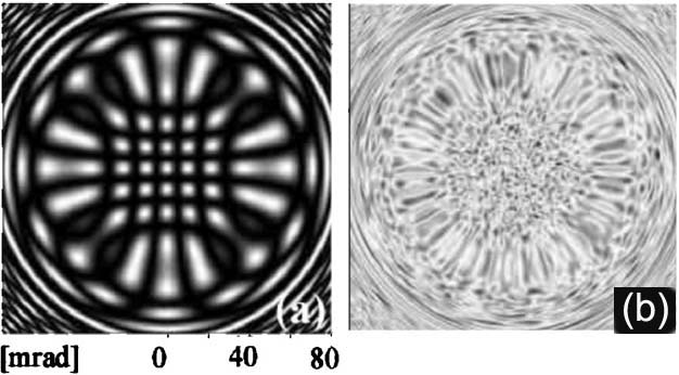
Figure 3590b. Simulated Ronchigrams with a spherical aberration of 10 µm and a defocus of -70 nm: (a) For lattice 0.7 nm lattice specimen and (b) For amorphous foil specimen.
Adapted from [10]
Figure 3590c shows the optical schematics of defocused TEM and STEM. The aberrations in STEM mode can be detected and corrected using the symmetry in the Ronchigram that includes the azimuthal and the radial circles of infinite magnification [4]. The solid lines represent the electron scattering direction at the radial circle in STEM mode, corresponding to the caustic curve in TEM mode. The azimuthal circle (broken line) is related to the angle of focusing on the specimen, i.e. part of the highly scattered electrons, which cross the optical axis on the specimen.
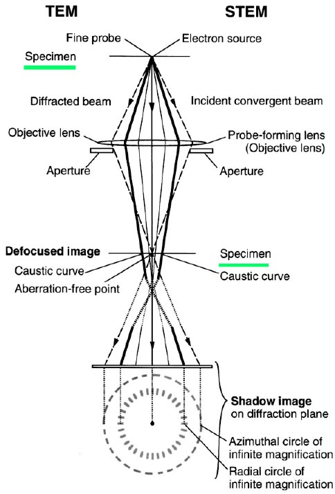
Figure 3590c. The optical schematics of defocused TEM and STEM. Adapted from [3]
It can be considered that the coma-free alignment in TEM mode corresponds to STEM alignment with Ronchigram in STEM mode, that is the Ronchigram can be used to detect coma aberration in a probe-forming lens (the objective lens in STEM) [2]. Therefore, the STEM coma-free alignment is carried out by coinciding the aperture center with the center of the azimuthal- or radial-circle. Note that the Ronchigram locates on the diffraction plane.
Table 3590. Equivalent functions in TEM and STEM modes.
In STEMs, the useful part of the Ronchigram is selected by VOAs (virtual objective apertures), probe forming aperture, or called “condenser aperture”. Figure 3590d (a) shows the coherent electron Ronchigram formed from an amorphous material. The interference pattern of the Ronchigram at the smooth center flashes randomly due to the small movements of the incident electron probe and specimen. If the sample is more than a few nm thick, the smooth region will be replaced by faint random mist because the top and bottom cannot be at infinite magnification at the same defocus. [5] Figure 3590d (b) shows a schematic illustration of the Ronchigram indicating the location of the rings caused by spherical aberration (Cs) and the shadow image inside the rings. The aperture size should be small enough in order to exclude these rings. However if a too small aperture is used the available high frequencies will not be included and the probe becomes diffraction limited. In practice, the probe-forming aperture marked by the red dotted circle in Figure 3590d (a) is just inside the consequence of the Cs rings.
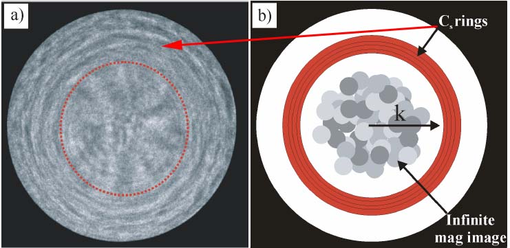
Figure 3590d (a) The coherent electron Ronchigram formed from an amorphous material, and (b) The rings caused by spherical aberration and the shadow image inside the rings. [5]
In STEM operation, to observe the Ronchigram, the apertures after the specimen are removed and a large probe convergence angle (>100 mrad) is selected, for instance by inserting the largest STEM objective aperture (condenser aperture in CTEM).
The main advantage of using a Ronchigram, e.g. in STEM mode, is that the coma-free axis is directly visible.
[1] J.M. Cowley, Electron diffraction phenomena observed with a high resolution STEM instrument, J. Electron. Microsc. Tech. 3 (1986) 25-44.
[2] J. A. Lin, J. M. Cowley, Ultramicroscopy 19 (1986) 31.
[3] Koji Kimoto, Kazuo Ishizuka, Nobuo Tanaka, Yoshio Matsui, Practical procedure for coma-free alignment using caustic figure, Ultramicroscopy 96 (2003) 219–227.
[4] N. Dellby, O.L. Krivanek, P.D. Nellist, P.E. Batson, A.R. Lupini, J. Electron Microsc. 50 (2001) 177.
[5] M. Weyland and D. A. Muller, Tuning the convergence angle for optimum STEM performance, FEI nanoSolutions, (2006) 24.
[6] J.M. Cowley, Ultramicroscopy 2 (1976) 3.
[7] J.M. Cowley, Ultramicroscopy 4 (1979) 435.
[8] Q.M. Ramase, A.L. Bleloh, Ultramicroscopy 106 (2005) 37.
[9] T. Yamazaki, Y. Kotaka, Y. Kikuchi, K. Watanabe, Ultramicroscopy 106 (2006)
153.
[10] Sawada H, Sannomiya T, Hosokawa F, Nakamichi T, Kaneyama T, Tomita T, Kondo Y, Tanaka T, Oshima Y, Tanishiro Y, and Takayanagi K (2008) Measurement method of aberration from Ronchigram by autocorrelation function. Ultramicroscopy 108: 1467–1475.
|