=================================================================================
Under the isoplanatic approximation as well as Taylor expansion, the wave aberration function, W, using the notation provided by Krivanek [1], can be concisely expanded to sixth order in k about the origin of zero scattering angle in terms of the coherent aberration coefficients, given by,
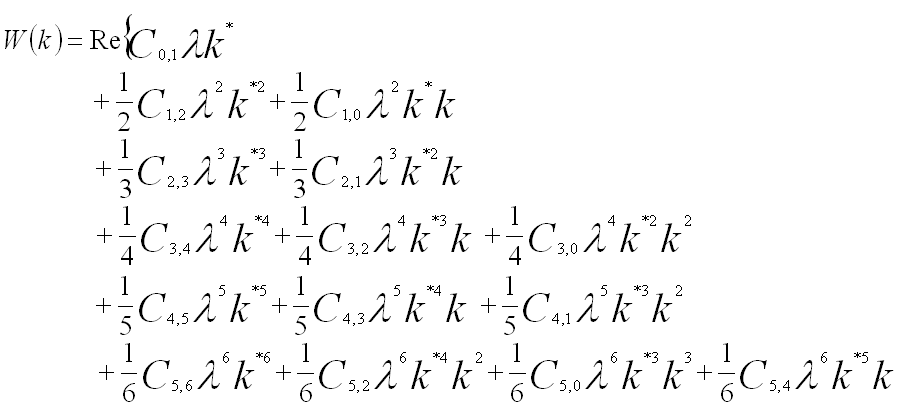
 ----------------------------------------------- [3740a] ----------------------------------------------- [3740a]
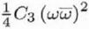
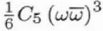
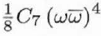
The first subscript refers to the order of the coefficient in terms of real space displacement, while the second subscript describes the angular symmetry. If the vector k is replaced by a complex number ω = λkx + iλky, the wave aberration function can be re-writen by,
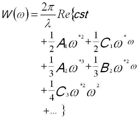 -------------------------------- [3740b] -------------------------------- [3740b]
The wave aberration function can also be expanded in polar notation. The following equation shows the terms to fourth order,
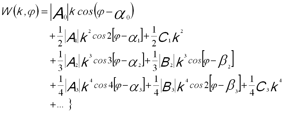 ----------- [3740c] ----------- [3740c]
The other way of presenting the wave aberration function at the back focal plane of a lens is based on polar angular coordinates θ and φ, given by,
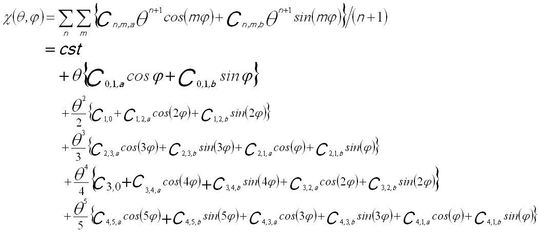
 --------------------------------------- [3740d] --------------------------------------- [3740d]
The sum over m is taken from 0 (or 1) to n+1 for each order n with the additional constraint that m+n is odd.
Table 3740a lists the aberration coefficient nomenclature, their order (of both the ray deviation (N) and the wavefront), and radial (azimuthal) symmetry. This table also compares both commonly used notations [1, 2]. The spherical aberration (highlighted in orange in Table 3740a) is always real and are usually the most significant among all the aberrations, while the off-axial coma (highlighted in green in Table 3740a) is complex in the presence of an axial magnetic field. Table 3740b also lists more different methods of axial aberration notations presented in different publications.
Table 3740a. Aberration Coefficient Nomenclature. The aberration coefficients have two
main types of notations, namely Krivanek notation, and Typke and Dierksen notation.
| Krivanek notation |
Haider[8] |
Radial Order |
Value |
Azimuthal Symmetry |
Wave aberration |
Nomenclature |
| Ray |
Wave
(k) |
| C0,1 |
|
0 |
1 |
Complex |
1 |
 |
Beam/image Shift |
| C1,2 |
A1 |
1 |
2 |
Complex |
2 |
 |
Two-fold axial astigmatism (or axial astigmatism of the 1st order) |
| C1,0 |
C1 |
1 |
2 |
Real |
0, ∞ |
 |
Defocus (overfocus positive, or spherical aberration of the 1st order; Real numbers and describing rotationally symmetric contributions to the wave aberration) (alt: Δf) |
| C2,3 |
A2 |
2 |
3 |
Complex |
3 |
 |
Three-fold axial astigmatism (or axial astigmatism of the 2nd order) |
| C2,1 |
B2 |
2 |
3 |
Complex |
1 |
 |
Second-order axial coma |
| C3,4 |
A3 |
|
4 |
Complex |
4 |
 |
Four-fold axial astigmatism or axial astigmatism of the 3rd order Cs |
| C3,2 |
S3 |
|
4 |
Complex |
2 |
 |
Twofold astigmatism of Cs (or Third order twofold astigmatism, or Axial star aberration of the 3rd order) |
| C3,0 |
C3 |
|
4 |
Real |
0, ∞ |
 |
Third-order spherical aberration (always positive for round lenses [3]; Real numbers and describing rotationally symmetric contributions to the wave aberration) (alt: Cs ) |
| C4,5 |
A4 |
|
5 |
Complex |
5 |
 |
Five-fold axial astigmatism or axial astigmatism of the 4th order |
| C4,1 |
B4 |
|
5 |
Complex |
1 |
 |
Fourth-order axial coma |
| C4,3 |
D4 |
4 |
5 |
Complex |
3 |
 |
Fourth order threefold astigmatism (or Three lobe aberration) |
| C5,4 |
R5 |
5 |
6 |
Complex |
4 |
 |
Fourfold astigmatism of C5 (or Fifth order rosette aberration) |
| C5,2 |
S5 |
5 |
6 |
Complex |
2 |
 |
Twofold astigmatism of C5 (or Fifth-order axial star aberration) |
| C5,0 |
C5 |
|
6 |
Real |
0, ∞ |
 |
Fifth-order spherical aberration |
| C5,6 |
A5 |
|
6 |
Complex |
6 |
 |
Six-fold axial astigmatism or sixfold axial astigmatism of the 5th order |
| C6,1 |
B6 |
|
|
Complex |
1 |
 |
Sixth order axial coma |
| C6,3 |
D6 |
|
|
Complex |
3 |
 |
Sixth order three-lobe aberration |
| C6,5 |
F6 |
|
|
Complex |
5 |
 |
Sixth order pentacle aberration |
| C6,7 |
A6 |
|
|
Complex |
7 |
 |
Sevenfold astigmatism |
| C7,0 |
C7 |
|
|
Real |
0 |
 |
Seventh-order spherical aberration |
| C7,2 |
S7 |
|
|
Complex |
2 |
 |
Seventh-order star aberration |
| C7,4 |
R7 |
|
|
Complex |
4 |
 |
Seventh-order rosette aberration |
| C7,6 |
G7 |
|
|
Complex |
6 |
 |
Seventh-order chaplet aberration |
| C7,8 |
A7 |
|
|
Complex |
8 |
 |
Eightfold astigmatism |
The indices n and k denote the order and azimuthal symmetry of the aberration Cn,k. In the equations above, Factors 1/(n+1) are used for all contributions to the nth order. [4] The aberration coefficients Cn,k are complex
numbers denoting the two Cartesian components except
C1,0(C1), C3,0(C3), and C5,0 that are real numbers. The aberration coefficients C1 and C3 describe rotationally symmetric contributions to the wave aberration. The complex coefficients involve both the strength and direction of the aberration. In the list in Table 3740a only the spherical aberration, C3, is completely unavoidable. C1 is almost always present since it is used to reduce the effects of the spherical aberration by slightly underfocusing the objective lens (corresponding to a negative C1). Without aberration corrections, the other aberrations usually are left out since they are much smaller then the two main aberrations C1 and C3. The wave aberration function can be separated into a symmetric part Ws with Ws = Ws-, e.g. containing the terms in A1, C1 and C3 and an antisymmetric part Wa with Wa = -Wa-, e.g. containing the terms in A2 and B2.
Table 3740b. Different methods of axial aberration notations presented in different publications.
| Krivanek[1] |
Typke and Dierksen[2] |
Sawada [5]* |
Zemlin [6] |
Isizuka[7] |
Haider[8] |
Pöhner and Rose |
Thust[9] |
| C0,1 |
A0 |
|
|
|
|
A0 |
|
| C1,2 |
A1 |
A2 |
a2 |
a2 |
A1 |
A1 |
C22 |
| C1,0 |
C1 |
O2 |
Δ |
z |
C1 |
C1 |
C20 |
| C2,3 |
A2 |
A3 |
a3 |
a3 |
A2 |
A2 |
C33 |
| (1/3)C2,1 |
B2 |
P3 |
b |
b |
B2 |
(1/3)B2 |
C31 |
| C3,4 |
A3 |
A4 |
|
|
A3 |
|
C44 |
| (1/4)C3,2 |
B3 |
Q4 |
|
|
S3 |
(1/4)B3 |
C42 |
| C3,0 |
C3 |
O4 |
Cs |
Cs |
C3 |
C3 |
C40 |
| C4,5 |
A4 |
A5 |
|
|
A4 |
|
C55 |
| (1/4)C4,1 |
B4 |
P5 |
|
|
B4 |
|
C51 |
| (1/4)C4,3 |
D4 |
R5 |
|
|
D4 |
(1/6)D5 |
C53 |
| (1/6)C5,4 |
R5 |
|
|
|
R5 |
|
|
| (1/6)C5,2 |
S5 |
|
|
|
S5 |
(1/6)B5 |
|
| C5,0 |
C5 |
O6 |
|
|
C5 |
C5 |
C60 |
| C5,6 |
A5 |
A6 |
|
|
A5 |
A5 |
C66 |
| |
D5 |
|
|
|
|
|
|
(1/7)C6,1 |
|
|
|
|
B6 |
|
|
(1/7)C6,3 |
|
|
|
|
D6 |
|
|
(1/7)C6,5 |
|
|
|
|
F6 |
|
|
| C6,7 |
|
|
|
|
A6 |
|
|
C7,0 |
|
|
|
|
C7 |
|
|
(1/8)C7,2 |
|
|
|
|
S7 |
|
|
(1/8)C7,4 |
|
|
|
|
R7 |
|
|
(1/8)C7,6 |
|
|
|
|
G7 |
|
|
| C7,8 |
|
|
|
|
A7 |
|
|
* "A" denotes the coefficient of the primary aberration, which is introduced by simple multi-pole field; "O" denotes round symmetry; "P" denotes one-fold symmetry; "Q" denotes tow-fold symmetry; "R" denotes three-fold symmetry; "S" denotes four-fold symmetry. The suffix number of the aberration coefficient corresponds to the order of the wave aberrations.
Figure 3740 shows the aberration coefficients from 0th to 5th order. The vertical lines indicate the groups of different angular symmetries, while the colors of the schematic illustrations in the same rows represent the order of the aberration coefficients. Corresponding to Equation 3740d, in Figure 3740 all the schematic illustrations represent the distortions of the electron wavefronts induced by axial geometric aberrations. The nth-order aberration-induced wavefront distortion on the diffraction plane increases with the distance (δ'r) from the optical axis by (n+1)th power (namely (δ'r)n+1) or increases with the angle (θ) by (n+1)th power (namely θn+1) in Equation 3740d, and the corresponding ray is displaced by nth power with distance δr (See Figure 3752a) on the image plane (namely δnr). The m index indicates the wavefront distortion repeats the maxima and mina m times for Cn,m when the coordinate system rotates for 360 degrees. The subscripts a and b represent that for the cases m > 0, the azimuthal variation of the aberrations have two orthogonal components, rotated by π/2m between Cn,m,a and Cn,m,b.
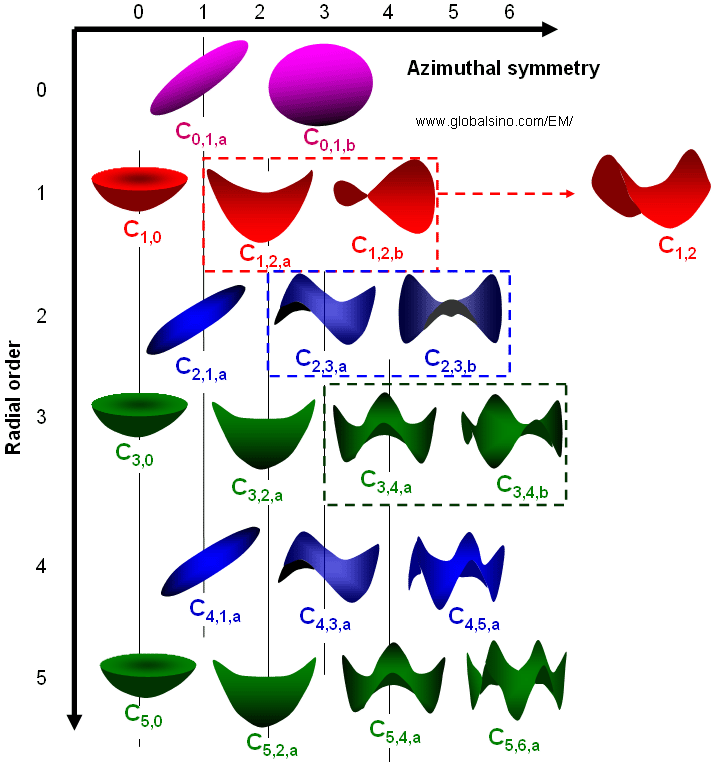
Figure 3740 shows the aberration coefficients from 0th to 5th order.
[1] Krivanek, O. L., Dellby, N., and Lupini, A. R. (1999). Towards sub-Å electron beams.
Ultramicroscopy 78, 1.
[2] Typke, D., and Dierksen, K. (1995). Determination of image aberrations in high-resolution
electron microscopy using diffractogram and cross correlation methods. Optik 99, 155.
[3] O. Scherzer, J. Appl. Phys. 20 (1949) 20.
[4] Saxton,W.O. (2000). A new way of measuring microscope aberrations. Ultramicroscopy 81, 41–45.
[5] H. Sawada, F. Hosokawa, T. Kaneyama, T. Tomita, Y. Kondo, T. Tanaka, Y.
Oshima, Y. Tanishiro, K. Takayanagi, Proc. Microsc. Microanal. 13 (2007) 880.
[6] F. Zemlin, K. Weiss, P. Schiske,W. Kunath, K.H. Herremann, Ultramicroscopy 3
(1978) 46.
[7] K. Ishizuka, Ultramicroscopy 55 (1994) 407.
[8] M. Haider, S. Uhlemann, J. Zach, Ultramicroscopy 81 (2000) 163.
[9] A. Thust, J. Barthel, L. Houben, C.L. Jia, M. Lentzen, K. Tillmann, K. Urban, Proc.
Microsc. Microanal. 11 (2005) 58.
|