Incident electrons in EMs can undergo deceleration in the Coulomb field of the specimen atoms. This is the positive field of the nucleus modified by the negative field of an electron cloud. When the incident electrons interact with the Coulomb field, the electrons are scattered inelastically, resulting in EDS background. The background is not linear, and a simple interpolation is not sufficient.

One of the most important factors for X-ray element analytical techniques is the minimum detection limit. A principal factor determining the detection limits and errors, as indicated in the list above, is the degree of continuous background in the measured X-ray spectra since the X-ray spectrum recorded by EDS systems is composed of both the characteristic peaks and continuum background. In general, the background of EDS map and profile originates from stray radiation in the EM column and bremsstrahlung X-rays. The bremsstrahlung from the projectile or secondary electrons and atomic bremsstrahlung are the most important sources of the continuous X-ray background. For heavier projectiles and higher electron energies, the Compton tails of the X-rays start to contribute extremely. The bremsstrahlung radiation depends slightly on energy, especially for thin specimens where multiple scatterings of the high-energy electron are negligible. For the same reason, the TEM-EDS background is normally lower than that of SEM-EDS on bulk materials (see page4532). However, in practice, the background becomes zero at the low end of the spectrum because of absorption by the detector dead layer and the detector window.

The background needs to be removed before the peak intensities are obtained. In the analysis of an EDS data, a power series in energy is normally used to model the background. Basically, there are two main methods to remove the background from the measured spectral distribution:
        i) Background modeling. In this method, a continuum energy-distribution function is either calculated or measured and then combined with a mathematical description of the detector response function. The resulting function is used to extract the background spectrum that is subtracted from the measured spectral distribution.
        ii) Background filtering.  In this method, the physics of X-ray production and emission is ignored and the background is considered as an undesirable signal. The effect of the background can be removed by mathematical filtering or modification of the frequency distribution of the spectrum, for instance, by digital filtering and Fourier analysis.

Some other techniques can also be used to subtract the background depending on the shapes of the peak and background. For instance:
        iii) At high X-ray energies where the background is fairly linear, subtracting an interpolated background is a reliable method to evaluate the intensity of the X-ray lines, for instance, in Figure 3918b, the net signal intensity is given by:
            P = S - (B1 + B2)•(2M + 1)/(2N) ---------------- 3918a
     Or,  P' = S/(2M + 1) - (B1 + B2)/(2N) ---------------- 3918b
It is important to note that, in this background subtraction method, the accuracy of background correction and the reproducibility of the results highly depends on the choice of points for fitting (B1 and B2 in Figure 3918b).

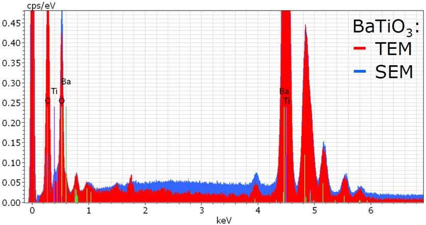
The peak integration can be done either by fitting a Gaussian profile or by using reference spectra that have been recorded previously and stored in the computer. If there is a peak overlap, it is better to deal with sets of peaks (e.g. K_α, K_β, L-series) with the energies and relative intensities between elements.

The background counts in TEM-EDS are much lower than those in SEM-EDS spectrum. Due to the high background counts in SEM-EDS, an artificial carbon (C) peak is always visible and thus a value of more than 2% carbon is normally measured even though there is no carbon in the specimen. This artefact is due to the window in the detector. The EDS windows are normally SATW windows and their material has a specific transmission profile with a strong absorption edge just above but very close to the C X-ray energy, resulting in an artificial peak at the C energy position. Therefore, it is the strong absorption of the background (continuum) X-rays that produces the artefact peak. Note that SATW detector windows are AP* ultrathin polymer windows manufactured by Moxtek and are almost supplied by all EDS detector companies. However, a TEM-EDS spectrum taken from the same specimen materials does not show such a artefact peak at the carbon energy because the spectrum consists mostly of characteristic X-rays.

There are basically two different methods used in EDS software to correct and subtract the background of EDX spectra as listed in Table 3918a. In modern EDS software, the background including many factors such as the collection efficiency of the detector, the processing efficiency of the detector and the absorption of X-ray within the specimen can be modeled. However, in practice, no software with different models can perform perfect subtraction of background. Therefore, it is very useful that the quantified results obtained from different software is compared.

Table 3918a. Background subtraction of EDX spectrum used in EDS software.

	Fit method
	Physical modeling	Mathematical method
Principle	Kramer’s law	Signal/noise filtering
NSS	Gaussian	Digital top hat filter
EDAX	Gaussian	Top-hat filter
Bruker [2]
	P/B-ZAF is optimized; OK for Phi-Rho-Z	Produces background curvatures at overlapping peaks; OK for Phi-Rho-Z
Particular applications	Ultra-light elements

It is necessary to highlight that except for the random errors from counting statistics, some factors, however, will contribute systematic errors. Those factors are mainly:
         i) The accuracy of the chemical composition of the standard (if calibration or correction of k_AB factors is applied).
         ii) The presence of spurious X-rays.
         iii) The inaccuracy of evaluation of the specimen thickness.
         iv) The deconvolution of overlapping peaks.
         v) Thee background-fitting routine.

Two approaches are normally used in EDS systems today:
         i) Automatically construct the background based on the known physics and proper corrections. This method is fast and lets the user to judge the quality of the model.
         ii) Manually model the background. In this case, the user makes his own background model by creating the correction form based on the automatic background points. In the manual background method, it is also possible to correct the different absorption edges of the materials.

Table 3918b. Some special cases of total background.

Line	Case	Total background
Kα	Sample with a light matrix like carbon (C)	Much less than 1 % of peak height for a pure element at any energy
Kα	Sample with heavier matrices like Fe	~ 1 wt%
Kα	samples with particularly heavy matrices like Au	several wt% at higher energies
Kα	At 5 kV of incident beam, with heavier matrices like Fe	For Cl Kα, background = ~3 wt%
Kα	At 20 kV of incident beam, with heavier matrices like Fe	For Cl Kα, background = ~0.6 wt%
L/M		Background effect is greater than for K lines, because the peak height for L or M lines is less than for K at the same concentration, so that the background correction has to be more accurate
L	Fe matrix	For Fe L line, background = ~10 wt%

[1] Ralf Terborg, Bruker.
[2] Quantification of EDS spectra, Bruker.
[3] Peter J. Statham, Limitations to Accuracy in Extracting Characteristic Line Intensities From X-Ray Spectra, J. Res. Natl. Inst. Stand. Technol. 107, 531–546 (2002).