| The top-hat and bottom-hat filtering techniques are useful for enhancing details in an image if shading is present. On the other hand, it is important that these filtering transformations can be used to correct the effects of non-uniform illumination since proper illumination plays a major role in the process of extracting objects from the background.
Top-hat filtering
The top-hat filtering, also called top-hat transformation operator or white-top-hat filtering, in the mathematical morphology estimates the trend via morphological opening and then removes
this trend from an image [1]. The morphological opening, and the thus top-hat filter,
works in the following steps:
i) Replaces each pixel by the minimum value of the pixels
in a square centered around it.
ii) Replaces each pixel with the maximum value in the window of the created image in step i).
iii) Subtracts the morphological opening, ϕ(f), from the original image, f:
Tophat(f) = f - (f  Y) ---------------------------------------------- [1004a] Y) ---------------------------------------------- [1004a]
= f - ϕ(f) ---------------------------------------------------- [1004b]
= Image - Open(Image) ---------------------------------- [1004c]
where,
f -- the original image,
-- the opening operator. The opening operator removes weak boundaries between objects and small details.
Y -- the structuring element,
ϕ(f) -- the subsequent maximum filter in step ii).
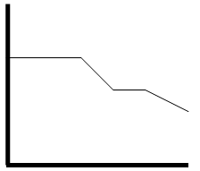
The top-hat filter has the property of enhancing "peaks" by applying the opening operator. It returns the difference between the result of morphological opening operation and the original data f. Figure 1004a shows a schematic of top-hat filtering. Such top hat filter is a ranking filter that compares the brightness of pixels in two different
neighborhoods around each location. The central region in blue is large enough to correspond to the
spike, while the outer region in red is an annulus surrounding the
central one, like the brim of a top hat (where the name is from). If the maximum value in the central
blue region exceeds that in the brim by more than a threshold, namely the
height of the hat, then a spike has been found. The inner and outer radii
of the brim and the height of the central
blue region are all adjustable parameters [7]. The filter can be used to locate either bright or dark
spots, as desired.

Figure 1004a. Schematic of top-hat filtering. |
Figure 1004b shows a simple example of top-hat filtering. The resulted image in Figure 1004b (c) is obtained by subtracting the image in Figure 1004b (b) from the original image in Figure 1004b (a), which is the opening operation process.
| Figure 1004b. Simple example of top-hat filtering: (a) Original image, (b) opening operator, (c) obtained image after the opening operation in (b). |
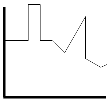
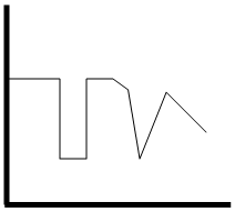
Figure 1004c shows an example of top-hat filtering applied to the pixel values in an more complicated one dimension (1-D) profile. The solid grey line
represents the raw pixel values obtained from an experiment, while the grey-filled shape shows the top-hat filtered values. The filtered values are obtained by subtracting the dotted black line from the original grey line.
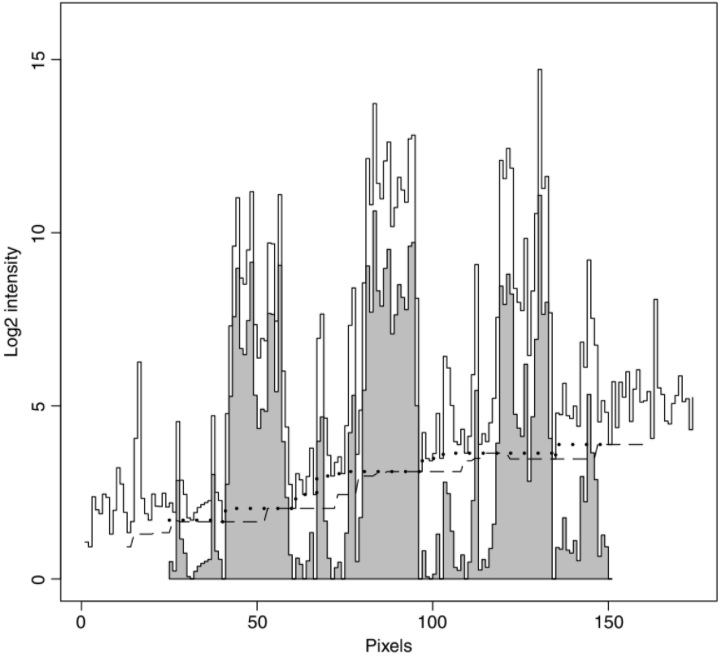
| Figure 1004c. One-dimensional top-hat filtering. The solid grey line
represents the raw pixel values obtained from an experient, the dashed black line is the minimum filter, the
dotted black line is the subsequent maximum filter, and the grey-filled line at the bottom
represents the top-hat filtered values. [2] |
It was suggested that choosing the window size appropriately for
top-hat filtering helps to reduce the across-array variance. [3] If the side width of the window is about  (d is the diameter of the spot), then the window will only
just cover the spot. In this case, very few background pixels will be sampled
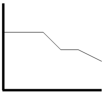
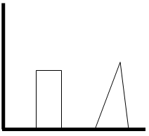
to choose the minimum pixel value, and thus the filter is less stable. Figure 1004d shows the visualization of changes in across-array standard deviation of top-hat
filtering as the filter window increases. At position C, the filtering becomes equivalent to constant background subtraction, and thus the standard deviation of the array remains unchanged. The optimum window size occurs at B, where
the filter reduces the standard deviation of spots across the array. Therefore, the choice of the window size is really important: (d is the diameter of the spot), then the window will only
just cover the spot. In this case, very few background pixels will be sampled
to choose the minimum pixel value, and thus the filter is less stable. Figure 1004d shows the visualization of changes in across-array standard deviation of top-hat
filtering as the filter window increases. At position C, the filtering becomes equivalent to constant background subtraction, and thus the standard deviation of the array remains unchanged. The optimum window size occurs at B, where
the filter reduces the standard deviation of spots across the array. Therefore, the choice of the window size is really important:
i) If it is too small, the background removal is then affected by the presence of random noise.
ii) If it is too large, then it cannot reproduce the small scale variations of the faint objects.
Therefore, a appropriate compromise has to be used.
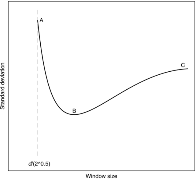
Figure 1004d. Visualization of changes in across-array standard deviation of top-hat
filtering as the filter window increases. The optimum window size occurs at B. [2] |
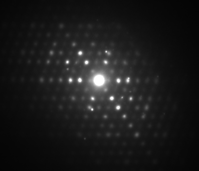
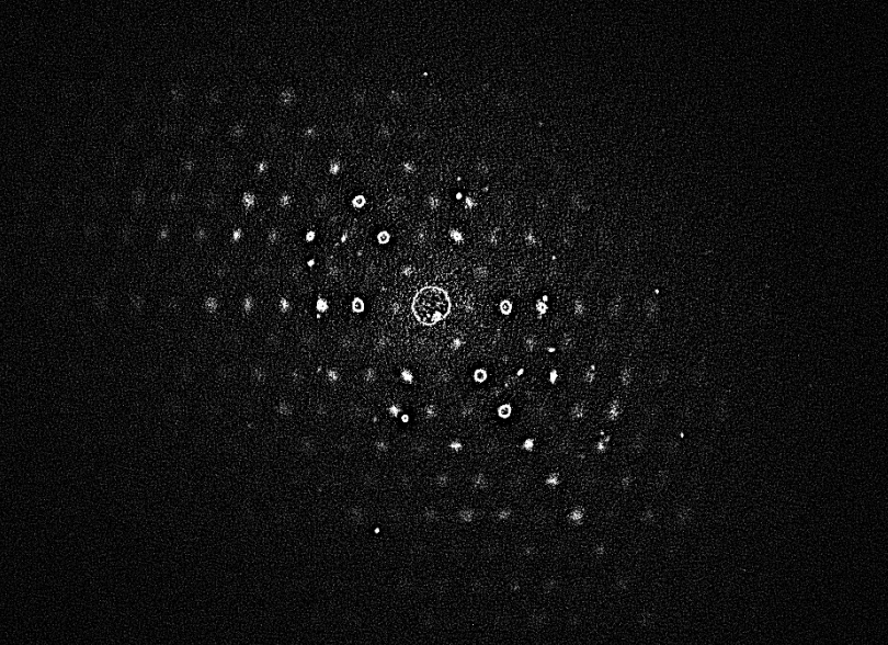
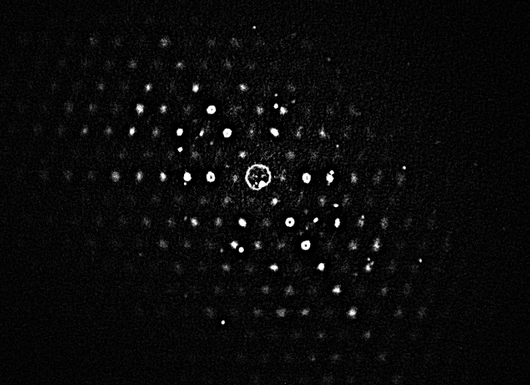
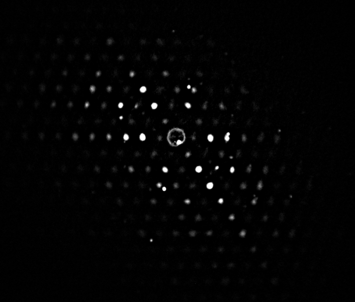
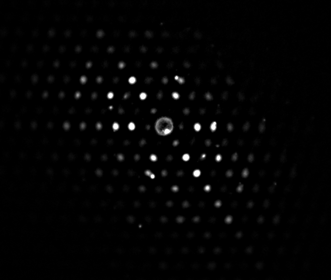
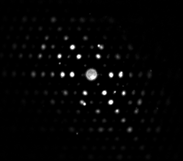
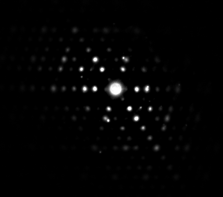
Figure 1004e shows the effect of the filter window (brim size, r) of top-hat filtering applied to an electron diffraction pattern. It can be seen that the background and noise are better removed with large brim sizes. However, the filtered diffraction pattern will not be correct if the brim size is too large.
◆ Script file
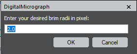
◆ Script lines used to change the brim size:

◆The pop-up window in script execution:
 |
 |
(a) |
(b) |
 |
 |
(c) |
(d) |
 |
 |
(e) |
(f) |
 |
 |
(g) |
(h) |
| Figure 1004e. Effect of filter window (brim size) of top-hat filtering applied to an electron diffraction pattern: (a) the script, (b) original diffraction pattern, (c) r = 2, (d) r = 4, (e) r = 8, (f) r = 16, (g) r = 32, and (h) r = 64. |
The top-hat filter technique has the following properties:
i) Strong background suppression effect.
ii) Smoothing effect.
The top-hat filter allows for the robust removal of slowly changing background on an array and has become an important tool in many image analysis applications, for instance:
i) Morphological sharpening.
ii) In dental image analysis, the top-hat filter is applied to enhance the bright regions that correspond to the teeth. [4]
iii) Detection of relatively small edges superimposed on large background signals in electron energy-loss spectroscopy (EELS).
[5]
iv) Removal of spikes in forensic images. [6]
v) Finding spikes in Fourier transform power spectra.
vi) Applied to spatial domain
images to find or remove features of a known size and minimum separation.
vii) Remove particles, which are darker than their surroundings, by replacing the pixels within the crown of the hat with a
value from the brim area. In this case, the process is sometimes called a rolling-ball
filter. The analogy is to roll a ball of specified diameter on the data. At any location where the
ball cannot touch the bottom of a pit, the values in the pit are replaced with values taken from
the surroundings.
viii) Quantitative analysis in EDS and EELS.
Bottom-hat filtering
The bottom-hat filtering, or called black-top-hat filtering, is given by,
Bottomhat(f) = (f  Y) - f ------------------------------------------- [1004d] Y) - f ------------------------------------------- [1004d]
= Close(Image) - Image ------------------------------------ [1004e]
where,
f -- the original image,
-- the closing operator.
The bottom-hat filter has the property of enhancing "valleys" by applying the closing operator. The resulted image in Figure 1004f (c) is obtained by subtracting the image in Figure 1004f (b) from the original image in Figure 1004f (a), which is the opening operation process.
| Figure 1004f. Simple example of top-hat filtering: (a) Original image, (b) opening operator, (c) obtained image after the opening operation in (b). |
The bottom-hat filter has many applications as well, for instance:
i) Morphological sharpening.
[1] C. Glasbey, Image analysis of a genotyping microarray experiment. Technical Report
01-07, Biomathematics and Statistics, Scotland, 2001.
[2] Ernst Wit and John McClure, Statistics for Microarrays: Design, Analysis and Inference, 2004.
[3] Yang YH, Buckley MJ, Dudoit S and Speed TP 2000 Comparison of methods for
image analysis on cDNA microarray data. Technical Report 584, Department
of Statistics, University of California, Berkeley, CA.
[4] K. Kamalanand, B. Thayumanavan, P. Mannar Jawahar, Computational Techniques for Dental Image Analysis (Advances in Medical Technologies and Clinical Practice (AMTCP)), 2018.
[5] Nestor J. ZALUZEC, Digital Filters for Application to Data Analysis in Electron Energy-Loss Spectrometry, Ultramicroscopy, 18, (1985), 185-190.
[6] John C. Russ, Forensic Uses of Digital Imaging, 2016.
[7] D. S. Bright, E. B. Steel. (1986). Bright field image correction with various image processing tools. In A. D.
Romig, ed., Microbeam Analysis 1986. San Francisco Press, San Francisco, CA, pp. 517–520.
|