| The energy scale and position of EELS should be routinely calibrated, especially for core-loss analysis. Depending on the edge availability in the specimen and standards, the reference edge for energy calibration can be different. The most common methods for EELS energy calibration are:
i) Calibrated against π* peak of K edge of amorphous carbon (C) because the C π* peak is accurately locked at 285 eV.
ii) Calibrated using the known threshold energy of the C K-edge of the amorphous C support film of the TEM grid.
iii) Calibrated with the π* peak at the B K edge, which occurs at 192.1 eV [8].
The near-edge fine structure (ELNES) of carbon varies with different carbon structures [1-7], which is not suitable for calibration.
Ideally, the detector channel of the zero-loss peak should be calibrated to the voltage offset applied to the spectrometer drift tube. However, it is not unusual that the energy stability is poor or there are spectral shifts due to magnetic fields so that the energy calibration is not reliable.
Note that the energy calibration and thus the selection of the energy windows affect the accuracy of mapping and quantification significantly in EELS measurements.
Post-data-acquisition calibration of the dispersion scale as well as energy of spectra obtained with DigitalMicrograph (DM) can be conveniently performed. Different version of DM has slightly different user interface but all their calibration processes use commands to make adjustments to the energy-scale calibration of the selected spectrum. Depending on the accuracy of the dispersion in the spectra, we can have two different methods for the calibration:
i) Calibrate using just one feature of known energy if the dispersion is known to high accuracy. This method is sometimes called partial calibration.
ii) Calibrate using two features of known energies if we do not know the dispersion accuracy or know it is inaccurate. This method is sometimes called full calibration.
Here, we use free version DM 3.10 as an example for Method i):
i) Ensure the spectrum of interest is front-most as shown in Figure 4338a. The spectrum of interest here is zero-loss peak. As we can know from the figure, the zero-loss peak has an off-set, which needs to be calibrated.
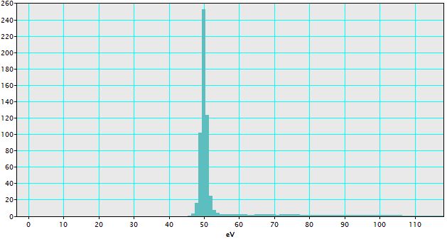
Figure 4338a. Zero-loss peak with an off-set. |
ii) Click once on the spectrum to place a single channel as shown in Figure 4338b.
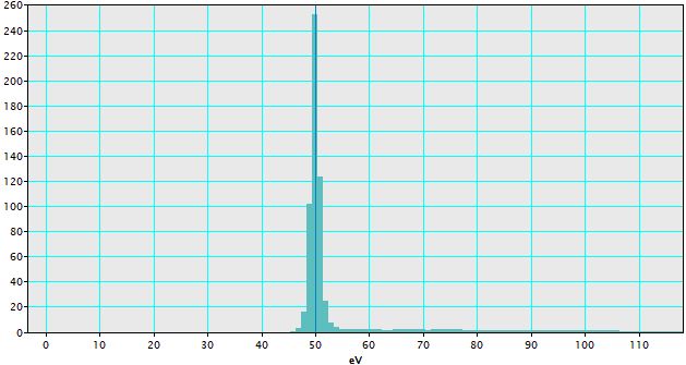
Figure 4338b. Zero-loss peak with an off-set, with a single channel in blue. |
iii) Select the Calibrate… menu item in the Spectrum menu.
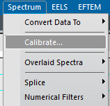
Figure 4338c. Select the Calibrate… menu item in the Spectrum menu. |
iv) Specify the ROI energy (0 eV since this is a zero loss peak)
and the known dispersion (1 eV/channel).
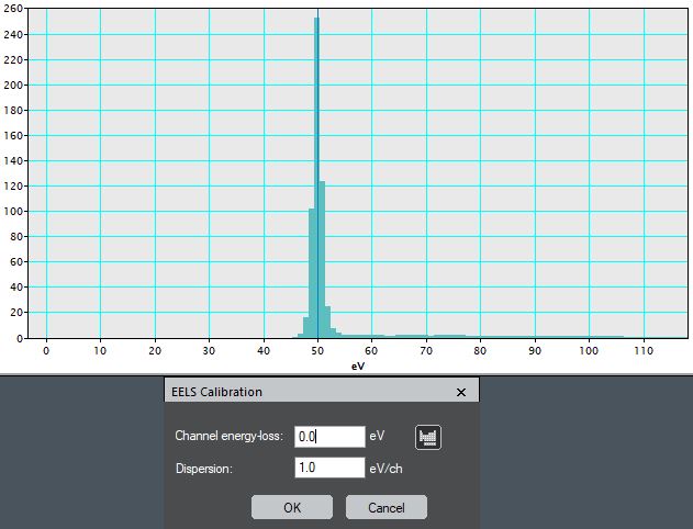
Figure 4338d. ROI energy (0 eV since this is a zero loss peak)
and the known dispersion (1 eV/channel). |
v) Click "OK", then the calibrated spectrum is obtained as shown in Figure 4338e. The zero-loss peak does not have off-set anymore.
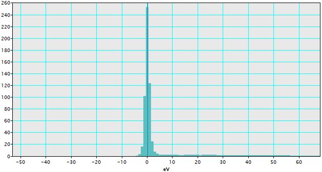
Figure 4338e. Calibrated spectrum. |
However, Method ii) can always be used no matter if the dispersion is accurate or not. Here, we still use DM 3.10 as an example:
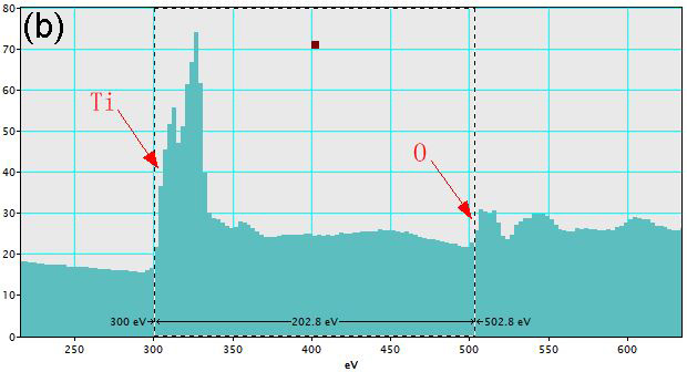
i) Ensure the spectrum of interest with two features of known energies is front-most. Figure 4338f shows a spectrum of TiO2 materials. In this figure, the edge of titanium (Ti) is at 300 eV and the edge of oxygen (O) is at 502.8 eV. The difference between the two edges is 202.8 eV. However, based on the EELS periodic table, all the three numbers are wrong. The error of the energy difference between the Ti and O edges indicates that the dispersion in the data acquisition software (DM normally) is inaccurate.
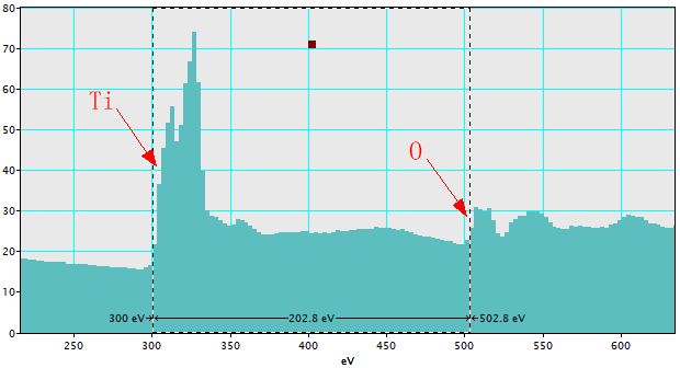
Figure 4338f. Spectrum of TiO2 materials before calibration. |
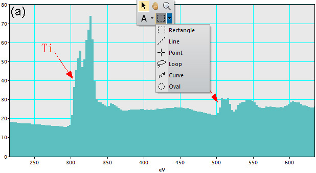
ii) Place a Rectangle ROI from Ti edge to O edge as shown in Figure 4338g. The two edges are the two reference points to be used in the
calibration procedure.
Figure 4338g. (a) Rectangle ROI function, and (b) Obtained Rectangle ROI from Ti edge to O edge. |
iii) Select the Calibrate… menu item in the Spectrum menu as shown in Figure 4338h.
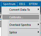
Figure 4338h. Calibrate… menu item in the Spectrum menu. |
iv) Specify the ROI start and
end energies as shown in Figure 4338i. Note that before performing the calibration, you will need to find the edges of the peaks of the corresponding elements from EELS periodic table. Here, we have Ti and O.
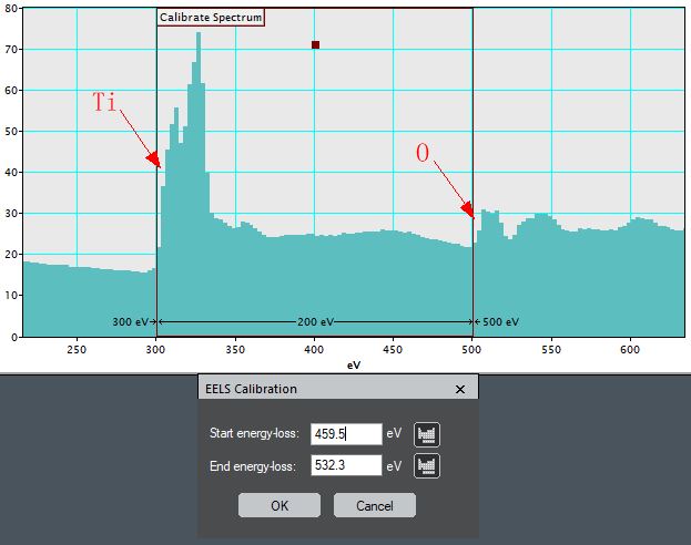
Figure 4338i. Specified ROI start and
end energies. Start energy: Ti edge (459.5 eV), and
End energy: O edge (532.3 eV). |
v) Click "OK", and then the calibrated spectrum in Figure 4338j is obtained.
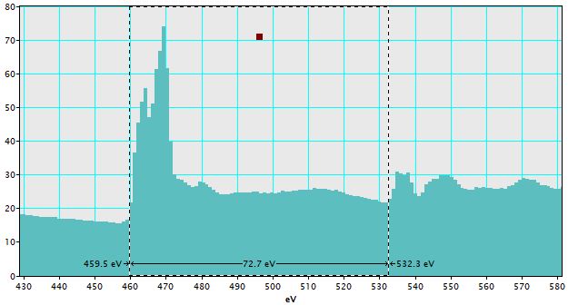
Figure 4338j. Calibrated spectrum. |
Table 4338 lists the edges of Ti and O and their energy difference before and after calibration.
Table 4338. The edges of Ti and O and their energy difference before and after calibration. |
| |
Ti (eV) |
O (eV) |
Difference (eV) |
| Before calibration |
300 |
502.8 |
202.8 |
| After calibration |
459.5 |
532.3 |
72.7 |
[1] P.E. Batson, Phys. Rev. B 48 (1993) 2608.
[2] P.A. Brühwiler, A. J. Maxwell, C. Puglia, A. Nilsson, S. Andersson, N. Martensson, Phys. Rev. Lett. 74 (1995) 614.
[3] K. Yase, S. Horiuchi, M. Kyotani, M. Yumura, K. Uchida, S. Ohshima, Y. Kuriki, F. Ikazaki, N. Yamahira, Thin Solid Films 273 (1996) 222.
[4] K. Suenaga, E. Sandre, C. Colliex, C. J. Pickard, H. Kataura, S. Iijima, Phys. Rev. B. 63 (2001) 165408.
[5] O. Stéphan, M. Kociak, L. Henrard, K. Suenaga, A. Gloter, M. Tence, E. Sandre, C. Colliex, J. Elec. Spec. 114-116 (2001) 209.
[6] J. Yuan and L. M. Brown, Micron 31 (2000) 515.
[7] I. Jimenez, R. Gago, J. M. Albella, Diamond and Related Materials 12 (2003) 110.
[8] Laurence A. J. Garvie, Peter R. Buseck, and Peter Rez, Characterization of Beryllium–Boron-Bearing Materials by Parallel Electron Energy-Loss Spectroscopy (PEELS), Journal of Solid State Chemistry 133, 347Ð355 (1997).
|